Convolutional layers literally perform convolution, which means applying several filters to the image to extract features. These filters are called kernels, and convolved images are called feature maps. Let's see the following image (decomposed to color values) and kernel:

With these, what is done with convolution is illustrated as follows:

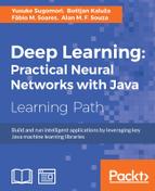
The kernel slides across the image and returns the summation of its values within the kernel as a multiplication filter. You might have noticed that you can extract many kinds of features by changing kernel values. Suppose you have kernels with values as described here:

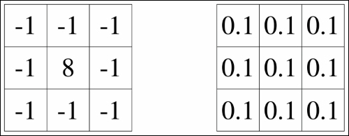
You see that the kernel on the left extracts the edges of the image because it accentuates the color differences, and the one on the right blurs the image because it degrades the original values. The great thing about CNN is that in convolutional layers, you don't have to set these kernel values manually. Once initialized, CNN itself will learn the proper values through the learning algorithm (which means parameters trained in CNN are the weights of kernels) and can classify images very precisely in the end.

Now, let's think about why neural networks with convolutional layers (kernels) can predict with higher precision rates. The key here is the local receptive field. In most layers in neural networks except CNN, all neurons are fully connected. This even causes slightly different data, for example, one-pixel parallel data would be regarded as completely different data in the network because this data is propagated to different neurons in hidden layers, whereas humans can easily understand they are the same. With fully connected layers, it is true that neural networks can recognize more complicated patterns, but at the same time they lack the ability to generalize and lack flexibility. In contrast, you can see that connections among neurons in convolutional layers are limited to their kernel size, making the model more robust to translated images. Thus, neural networks with their receptive fields limited locally are able to acquire translation invariance when kernels are optimized.

Each kernel has its own values and extracts respective features from the image. Please bear in mind that the number of feature maps and the number of kernels are always the same, which means if we have 20 kernels, we have also twenty feature maps, that is, convolved images. This can be confusing, so let's explore another example. Given a gray-scaled image and twenty kernels, how many feature maps are there? The answer is twenty. These twenty images will be propagated to the next layer. This is illustrated as follows:

So, how about this: suppose we have a 3-channeled image (for example, an RGB image) and the number of kernels is twenty, how many feature maps will there be? The answer is, again, twenty. But this time, the process of convolution is different from the one with gray-scaled, that is 1-channeled, images. When the image has multiple channels, kernels will be adapted separately for each channel. Therefore, in this case, we will have a total of 60 convolved images first, composed of twenty mapped images for each of the 3 channels. Then, all the convolved images originally from the same image will be combined into one feature map. As a result, we will have twenty feature maps. In other words, images are decomposed into different channeled data, applied kernels, and then combined into mixed-channeled images again. You can easily imagine from the flow in the preceding diagram that when we apply a kernel to a multi-channeled image to make decomposed images, the same kernel should be applied. This flow can be seen in the following figure:

Computationally, the number of kernels is represented with the dimension of the weights' tensor. You'll see how to implement this later.

What pooling layers do is rather simple compared to convolutional layers. They actually do not train or learn by themselves but just downsample images propagated from convolutional layers. Why should we bother to do downsampling? You might think it may lose some significant information from the data. But here, again, as with convolutional layers, this process is necessary to make the network keep its translation invariance.

There are several ways of downsampling, but among them, max-pooling is the most famous. It can be represented as follows:

In a max-pooling layer, the input image is segmented into a set of non-overlapping sub-data and the maximum value is output from each data. This process not only keeps its translation invariance but also reduces the computation for the upper layers. With convolution and pooling, CNN can acquire robust features from the input.

Now we know what convolution and max-pooling are, let's describe the whole model with equations. We'll use the figure of convolution below in equations:

As shown in the figure, if we have an image with a size of and kernels with a size of , the convolution can be represented as:

Here, is the weight of the kernel, that is, the model parameter. Just bear in mind we've described each summation from 0, not from 1, so you get a better understanding. The equation, however, is not enough when we think about multi-convolutional layers because it does not have the information from the channel. Fortunately, it's not difficult because we can implement it just by adding one parameter to the kernel. The extended equation can be shown as:

Here, denotes the channel of the image. If the number of kernels is and the number of channels is , we have . Then, you can see from the equation that the size of the convolved image is .

After the convolution, all the convolved values will be activated by the activation function. We'll implement CNN with the rectifier—the most popular function these days—but you may use the sigmoid function, the hyperbolic tangent, or any other activation functions available instead. With the activation, we have:

Here, denotes the bias, the other model parameter. You can see that doesn't have subscripts of and , that is, we have , a one-dimensional array. Thus, we have forward-propagated the values of the convolutional layer.

Next comes the max-pooling layer. The propagation can simply be written as follows:

Here, and are the size of pooling filter and . Usually, and are set to the same value of 2 ~ 4.

These two layers, the convolutional layer and the max-pooling layer, tend to be arrayed in this order, but you don't necessarily have to follow it. You can put two convolutional layers before max-pooling, for example. Also, while we put the activation right after the convolution, sometimes it is set after the max-pooling instead of the convolution. For simplicity, however, we'll implement CNN with the order and sequence of convolution–activation–max-pooling.

The simple MLP follows after convolutional layers and max-pooling layers to classify the data. Here, since MLP can only accept one-dimensional data, we need to flatten the downsampled data as preprocessing to adapt it to the input layer of MLP. The extraction of features was completed before MLP, so formatting the data into one dimension won't be a problem. Thus, CNN can classify the image data once the model is optimized. To do this, as with other neural networks, the backpropagation algorithm is applied to CNN to train the model. We won't mention the equation related to MLP here.

The error from the input layer of MLP is backpropagated to the max-pooling layer, and this time it is unflattened to two dimensions to be adapted properly to the model. Since the max-pooling layer doesn't have model parameters, it simply backpropagates the error to the previous layer. The equation can be described as follows:

Here, denotes the evaluation function. This error is then backpropagated to the convolutional layer, and with it we can calculate the gradients of the weight and the bias. Since the activation with the bias comes before the convolution when backpropagating, let's see the gradient of the bias first, as follows:

To proceed with this equation, we define the following:

We also define:

With these, we get:

We can calculate the gradient of the weight (kernel) in the same way:

Thus, we can update the model parameters. If we have just one convolutional and max-pooling layer, the equations just given are all that we need. When we think of multi-convolutional layers, however, we also need to calculate the error of the convolutional layers. This can be represented as follows:

Here, we get:

So, the error can be written as follows:

We have to be careful when calculating this because there's a possibility of or , where there's no element in between the feature maps. To solve this, we need to add zero paddings to the top-left edges of them. Then, the equation is simply a convolution with the kernel flipped along both axes. Though the equations in CNN might look complicated, they are just a pile of summations of each parameter.

With all the previous equations, we can now implement CNN, so let's see how we do it. The package structure is as follows:

ConvolutionNeuralNetworks.java is used to build the model outline of CNN, and the exact algorithms for training in the convolutional layers and max-pooling layers, forward propagations, and backpropagations are written in ConvolutionPoolingLayer.java. In the demo, we have the original image size of 12 12 with one channel:

final int[] imageSize = {12, 12};
final int channel = 1;

The image will be propagated through two ConvPoolingLayer (convolutional layers and max-pooling layers). The number of kernels in the first layer is set to 10 with the size of 3 3 and 20 with the size of 2 2 in the second layer. The size of the pooling filters are both set to 2 2:

int[] nKernels = {10, 20};
int[][] kernelSizes = { {3, 3}, {2, 2} };
int[][] poolSizes = { {2, 2}, {2, 2} };

After the second max-pooling layer, there are 20 feature maps with the size of 2 2. These maps are then flattened to 80 units and will be forwarded to the hidden layer with 20 neurons:

int nHidden = 20;

We then create simple demo data of three patterns with a little noise. We'll leave out the code to create demo data here. If we illustrate the data, here is an example of it:

Now let's build the model. The constructor is similar to other deep learning models and rather simple. We construct multi ConvolutionPoolingLayers first. The size for each layer is calculated in the method:

// construct convolution + pooling layers
for (int i = 0; i < nKernels.length; i++) {
   int[] size_;
   int channel_;

   if (i == 0) {
       size_ = new int[]{imageSize[0], imageSize[1]};
       channel_ = channel;
   } else {
       size_ = new int[]{pooledSizes[i-1][0], pooledSizes[i-1][1]};
       channel_ = nKernels[i-1];
   }

   convolvedSizes[i] = new int[]{size_[0] - kernelSizes[i][0] + 1, size_[1] - kernelSizes[i][1] + 1};
   pooledSizes[i] = new int[]{convolvedSizes[i][0] / poolSizes[i][0], convolvedSizes[i][1] / poolSizes[i][0]};

   convpoolLayers[i] = new ConvolutionPoolingLayer(size_, channel_, nKernels[i], kernelSizes[i], poolSizes[i], convolvedSizes[i], pooledSizes[i], rng, activation);
}

When you look at the constructor of the ConvolutionPoolingLayer class, you can see how the kernel and the bias are defined:

if (W == null) {

   W = new double[nKernel][channel][kernelSize[0]][kernelSize[1]];

   double in_ = channel * kernelSize[0] * kernelSize[1];
   double out_ = nKernel * kernelSize[0] * kernelSize[1] / (poolSize[0] * poolSize[1]);
   double w_ = Math.sqrt(6. / (in_ + out_));

   for (int k = 0; k < nKernel; k++) {
       for (int c = 0; c < channel; c++) {
           for (int s = 0; s < kernelSize[0]; s++) {
               for (int t = 0; t < kernelSize[1]; t++) {
                   W[k][c][s][t] = uniform(-w_, w_, rng);
               }
           }
       }
   }
}

if (b == null) b = new double[nKernel];

Next comes the construction of MLP. Don't forget to flatten the downsampled data when passing through them:

// build MLP
flattenedSize = nKernels[nKernels.length-1] * pooledSizes[pooledSizes.length-1][0] * pooledSizes[pooledSizes.length-1][1];

// construct hidden layer
hiddenLayer = new HiddenLayer(flattenedSize, nHidden, null, null, rng, activation);

// construct output layer
logisticLayer = new LogisticRegression(nHidden, nOut);

Once the model is built, we need to train it. In the train method, we cache all the forward-propagated data so that we can utilize it when backpropagating:

// cache pre-activated, activated, and downsampled inputs of each convolution + pooling layer for backpropagation
List<double[][][][]> preActivated_X = new ArrayList<>(nKernels.length);
List<double[][][][]> activated_X = new ArrayList<>(nKernels.length);
List<double[][][][]> downsampled_X = new ArrayList<>(nKernels.length+1);  // +1 for input X
downsampled_X.add(X);

for (int i = 0; i < nKernels.length; i++) {
   preActivated_X.add(new double[minibatchSize][nKernels[i]][convolvedSizes[i][0]][convolvedSizes[i][1]]);
   activated_X.add(new double[minibatchSize][nKernels[i]][convolvedSizes[i][0]][convolvedSizes[i][1]]);
   downsampled_X.add(new double[minibatchSize][nKernels[i]][convolvedSizes[i][0]][convolvedSizes[i][1]]);
}

preActivated_X is defined for convolved feature maps, activated_X for activated features, and downsampled_X for downsampled features. We put and cache the original data into downsampled_X. The actual training begins with forward propagation through convolution and max-pooling:

// forward convolution + pooling layers
double[][][] z_ = X[n].clone();
for (int i = 0; i < nKernels.length; i++) {
   z_ = convpoolLayers[i].forward(z_, preActivated_X.get(i)[n], activated_X.get(i)[n]);
   downsampled_X.get(i+1)[n] = z_.clone();
}

The forward method of ConvolutionPoolingLayer is simple and consists of convolve and downsample. The convolve function does the convolution, and downsample does the max-pooling:

public double[][][] forward(double[][][] x, double[][][] preActivated_X, double[][][] activated_X) {

   double[][][] z = this.convolve(x, preActivated_X, activated_X);
   return  this.downsample(z);

The values of preActivated_X and activated_X are set inside the convolve method. You can see that the method simply follows the equations explained previously:

public double[][][] convolve(double[][][] x, double[][][] preActivated_X, double[][][] activated_X) {

   double[][][] y = new double[nKernel][convolvedSize[0]][convolvedSize[1]];

   for (int k = 0; k < nKernel; k++) {
       for (int i = 0; i < convolvedSize[0]; i++) {
           for(int j = 0; j < convolvedSize[1]; j++) {

               double convolved_ = 0.;

               for (int c = 0; c < channel; c++) {
                   for (int s = 0; s < kernelSize[0]; s++) {
                       for (int t = 0; t < kernelSize[1]; t++) {
                           convolved_ += W[k][c][s][t] * x[c][i+s][j+t];
                       }
                   }
               }

               // cache pre-activated inputs
               preActivated_X[k][i][j] = convolved_ + b[k];
               activated_X[k][i][j] = this.activation.apply(preActivated_X[k][i][j]);
               y[k][i][j] = activated_X[k][i][j];
           }
       }
   }

   return y;
}

The downsample method follows the equations as well:

public double[][][] downsample(double[][][] x) {

   double[][][] y = new double[nKernel][pooledSize[0]][pooledSize[1]];

   for (int k = 0; k < nKernel; k++) {
       for (int i = 0; i < pooledSize[0]; i++) {
           for (int j = 0; j < pooledSize[1]; j++) {

               double max_ = 0.;

               for (int s = 0; s < poolSize[0]; s++) {
                   for (int t = 0; t < poolSize[1]; t++) {

                       if (s == 0 && t == 0) {
                           max_ = x[k][poolSize[0]*i][poolSize[1]*j];
                           continue;
                       }
                       if (max_ < x[k][poolSize[0]*i+s][poolSize[1]*j+t]) {
                           max_ = x[k][poolSize[0]*i+s][poolSize[1]*j+t];
                       }
                   }
               }

               y[k][i][j] = max_;
           }
       }
   }

   return y;
}

You might think we've made some mistake here because there are so many for loops in these methods, but actually there's nothing wrong. As you can see from the equations of CNN, the algorithm requires many loops because it has many parameters. The code here works well, but practically, you could define and move the part of the innermost loops to other methods. Here, to get a better understanding, we've implemented CNN with many nested loops so that we can compare the code with equations. You can see now that CNN requires a lot of time to get results.

After we downsample the data, we need to flatten it:

// flatten output to make it input for fully connected MLP
double[] x_ = this.flatten(z_);
flattened_X[n] = x_.clone();

The data is then forwarded to the hidden layer:

// forward hidden layer
Z[n] = hiddenLayer.forward(x_);

Multi-class logistic regression is used in the output layer and the delta is then backpropagated to the hidden layer:

// forward & backward output layer
dY = logisticLayer.train(Z, T, minibatchSize, learningRate);

// backward hidden layer
dZ = hiddenLayer.backward(flattened_X, Z, dY, logisticLayer.W, minibatchSize, learningRate);

// backpropagate delta to input layer
for (int n = 0; n < minibatchSize; n++) {
   for (int i = 0; i < flattenedSize; i++) {
       for (int j = 0; j < nHidden; j++) {
           dX_flatten[n][i] += hiddenLayer.W[j][i] * dZ[n][j];
       }
   }

   dX[n] = unflatten(dX_flatten[n]);  // unflatten delta
}

// backward convolution + pooling layers
dC = dX.clone();
for (int i = nKernels.length-1; i >= 0; i--) {
   dC = convpoolLayers[i].backward(downsampled_X.get(i), preActivated_X.get(i), activated_X.get(i), downsampled_X.get(i+1), dC, minibatchSize, learningRate);
}

The backward method of ConvolutionPoolingLayer is the same as forward, also simple. Backpropagation of max-pooling is written in upsample and that of convolution is in deconvolve:

public double[][][][] backward(double[][][][] X, double[][][][] preActivated_X, double[][][][] activated_X, double[][][][] downsampled_X, double[][][][] dY, int minibatchSize, double learningRate) {

   double[][][][] dZ = this.upsample(activated_X, downsampled_X, dY, minibatchSize);
   return this.deconvolve(X, preActivated_X, dZ, minibatchSize, learningRate);

}

What upsample does is just transfer the delta to the convolutional layer:

public double[][][][] upsample(double[][][][] X, double[][][][] Y, double[][][][] dY, int minibatchSize) {

   double[][][][] dX = new double[minibatchSize][nKernel][convolvedSize[0]][convolvedSize[1]];

   for (int n = 0; n < minibatchSize; n++) {

       for (int k = 0; k < nKernel; k++) {
           for (int i = 0; i < pooledSize[0]; i++) {
               for (int j = 0; j < pooledSize[1]; j++) {

                   for (int s = 0; s < poolSize[0]; s++) {
                       for (int t = 0; t < poolSize[1]; t++) {

                           double d_ = 0.;

                           if (Y[n][k][i][j] == X[n][k][poolSize[0]*i+s][poolSize[1]*j+t]) {
                               d_ = dY[n][k][i][j];
                           }

                           dX[n][k][poolSize[0]*i+s][poolSize[1]*j+t] = d_;
                       }
                   }
               }
           }
       }
   }

   return dX;
}

In deconvolve, we need to update the model parameter. Since we train the model with mini-batches, we calculate the summation of the gradients first:

// calc gradients of W, b
for (int n = 0; n < minibatchSize; n++) {
   for (int k = 0; k < nKernel; k++) {

       for (int i = 0; i < convolvedSize[0]; i++) {
           for (int j = 0; j < convolvedSize[1]; j++) {

               double d_ = dY[n][k][i][j] * this.dactivation.apply(Y[n][k][i][j]);

               grad_b[k] += d_;

               for (int c = 0; c < channel; c++) {
                   for (int s = 0; s < kernelSize[0]; s++) {
                       for (int t = 0; t < kernelSize[1]; t++) {
                           grad_W[k][c][s][t] += d_ * X[n][c][i+s][j+t];
                       }
                   }
               }
           }
       }
   }
}

Then, update the weight and the bias using these gradients:

// update gradients
for (int k = 0; k < nKernel; k++) {
   b[k] -= learningRate * grad_b[k] / minibatchSize;

   for (int c = 0; c < channel; c++) {
       for (int s = 0; s < kernelSize[0]; s++) {
           for(int t = 0; t < kernelSize[1]; t++) {
               W[k][c][s][t] -= learningRate * grad_W[k][c][s][t] / minibatchSize;
           }
       }
   }
}

Unlike other algorithms, we have to calculate the parameters and delta discretely in CNN:

// calc delta
for (int n = 0; n < minibatchSize; n++) {
   for (int c = 0; c < channel; c++) {
       for (int i = 0; i < imageSize[0]; i++) {
           for (int j = 0; j < imageSize[1]; j++) {

               for (int k = 0; k < nKernel; k++) {
                   for (int s = 0; s < kernelSize[0]; s++) {
                       for (int t = 0; t < kernelSize[1]; t++) {

                           double d_ = 0.;

                           if (i - (kernelSize[0] - 1) - s >= 0 && j - (kernelSize[1] - 1) - t >= 0) {
                               d_ = dY[n][k][i-(kernelSize[0]-1)-s][j-(kernelSize[1]-1)-t] * this.dactivation.apply(Y[n][k][i- (kernelSize[0]-1)-s][j-(kernelSize[1]-1)-t]) * W[k][c][s][t];
                           }

                           dX[n][c][i][j] += d_;
                       }
                   }
               }
           }
       }
   }
}

Now we train the model, so let's go on to the test part. The method for testing or prediction simply does the forward propagation, just like the other algorithms:

public Integer[] predict(double[][][] x) {

   List<double[][][]> preActivated = new ArrayList<>(nKernels.length);
   List<double[][][]> activated = new ArrayList<>(nKernels.length);

   for (int i = 0; i < nKernels.length; i++) {
       preActivated.add(new double[nKernels[i]][convolvedSizes[i][0]][convolvedSizes[i][1]]);
       activated.add(new double[nKernels[i]][convolvedSizes[i][0]][convolvedSizes[i][1]]);
   }

   // forward convolution + pooling layers
   double[][][] z = x.clone();
   for (int i = 0; i < nKernels.length; i++) {
       z = convpoolLayers[i].forward(z, preActivated.get(i), activated.get(i));
   }


   // forward MLP
   return logisticLayer.predict(hiddenLayer.forward(this.flatten(z)));
}

Congratulations! That's all for CNN. Now you can run the code and see how it works. Here, we have CNN with two-dimensional data as input, but CNN can also have three-dimensional data if we expand the model. We can expect its application in medical fields, for example, finding malignant tumors from 3D-scanned data of human brains.

The process of convolution and pooling was originally invented by LeCun et al. in 1998 (http://yann.lecun.com/exdb/publis/pdf/lecun-98.pdf), yet as you can see from the codes, it requires much calculation. We can assume that this method might not have been suitable for practical applications with computers at the time, not to mention making it deep. The reason CNN has gained more attention recently is probably because the power and capacity of computers has greatly developed. But still, we can't deny the problem. Therefore, it seems practical to use GPU, not CPU, when we have CNN with certain amounts of data. Since the implementation to optimize the algorithm to GPU is complicated, we won't write the codes here. Instead, in Chapter 5, Exploring Java Deep Learning Libraries – DL4J, ND4J, and More and Chapter 7, Other Important Deep Learning Libraries, you'll see the library of deep learning that is capable of utilizing GPU.