TensorFlow is the library for machine learning and deep learning developed by Google. The project page is https://www.tensorflow.org/ and all the code is open to the public on GitHub at https://github.com/tensorflow/tensorflow. TensorFlow itself is written with C++, but it provides a Python and C++ API. We focus on Python implementations in this book. The installation can be done with pip, virtualenv, or docker. The installation guide is available at https://www.tensorflow.org/versions/master/get_started/os_setup.html. After the installation, you can import and use TensorFlow by writing the following code:

import tensorflow as tf

TensorFlow recommends you implement deep learning code with the following three parts:

We'll follow this guideline. A tutorial on MNIST classifications for beginners is introduced on https://www.tensorflow.org/versions/master/tutorials/mnist/beginners/index.html and the code for this tutorial can be found in DLWJ/src/resources/tensorflow/1_1_mnist_simple.py. Here, we consider refining the code introduced in the tutorial. You can see all the code in DLWJ/src/resources/tensorflow/1_2_mnist.py.

First, what we have to consider is fetching the MNIST data. Thankfully, TensorFlow also provides the code to fetch the data in https://github.com/tensorflow/tensorflow/blob/master/tensorflow/examples/tutorials/mnist/input_data.py and we put the code into the same directory. Then, by writing the following code, you can import the MNIST data:

import input_data

MNIST data can be imported using the following code:

mnist = input_data.read_data_sets("MNIST_data/", one_hot=True)

Similar to Theano, we define the variable with no actual values as the placeholder:

x_placeholder = tf.placeholder("float", [None, 784])
label_placeholder = tf.placeholder("float", [None, 10])

Here, 784 is the number of units in the input layer and 10 is the number in the output layer. We do this because the values in the placeholder change in accordance with the mini-batches. Once you define the placeholder you can move on to the model building and training. We set the non-linear activation with the softmax function in inference() here:

def inference(x_placeholder):

    W = tf.Variable(tf.zeros([784, 10]))
    b = tf.Variable(tf.zeros([10]))

    y = tf.nn.softmax(tf.matmul(x_placeholder, W) + b)

    return y

Here, W and b are the parameters of the model. The loss function, that is, the cross_entropy function, is defined in loss() as follows:

def loss(y, label_placeholder):
    cross_entropy = - tf.reduce_sum(label_placeholder * tf.log(y))

    return cross_entropy

With the definition of inference() and loss(), we can train the model by writing the following code:

def training(loss):
    train_step = tf.train.GradientDescentOptimizer(0.01).minimize(loss)

    return train_step

GradientDescentOptimizer() applies the gradient descent algorithm. But be careful, as this method just defines the method of training and the actual training has not yet been executed. TensorFlow also supports AdagradOptimizer(), MemontumOptimizer(), and other major optimizing algorithms.

The code and methods explained previously are to define the model. To execute the actual training, you need to initialize a session of TensorFlow:

init = tf.initialize_all_variables()
sess.run(init)

Then we train the model with mini-batches. All the data in a mini-batch is stored in feed_dict and then used in sess.run():

for i in range(1000):
    batch_xs, batch_ys = mnist.train.next_batch(100)
    feed_dict = {x_placeholder: batch_xs, label_placeholder: batch_ys}

    sess.run(train_step, feed_dict=feed_dict)

That's it for the model training. It's very simple, isn't it? You can show the result by writing the following code:

def res(y, label_placeholder, feed_dict):
    correct_prediction = tf.equal(
        tf.argmax(y, 1), tf.argmax(label_placeholder, 1)
    )

    accuracy = tf.reduce_mean(
        tf.cast(correct_prediction, "float")
    )

   print sess.run(accuracy, feed_dict=feed_dict)

TensorFlow makes it super easy to implement deep learning and it is very useful. Furthermore, TensorFlow has another powerful feature, TensorBoard, to visualize deep learning. By adding a few lines of code to the previous code snippet, we can use this useful feature.

Let's see how the model is visualized first. The code is in DLWJ/src/resources/tensorflow/1_3_mnist_TensorBoard.py, so simply run it. After you run the program, type the following command:

$ tensorboard --logdir=<ABOSOLUTE_PATH>/data

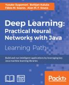
Here, <ABSOLUTE_PATH> is the absolute path of the program. Then, if you access http://localhost:6006/ in your browser, you can see the following page:

This shows the process of the value of cross_entropy. Also, when you click GRAPH in the header menu, you see the visualization of the model:

When you click on inference on the page, you can see the model structure:

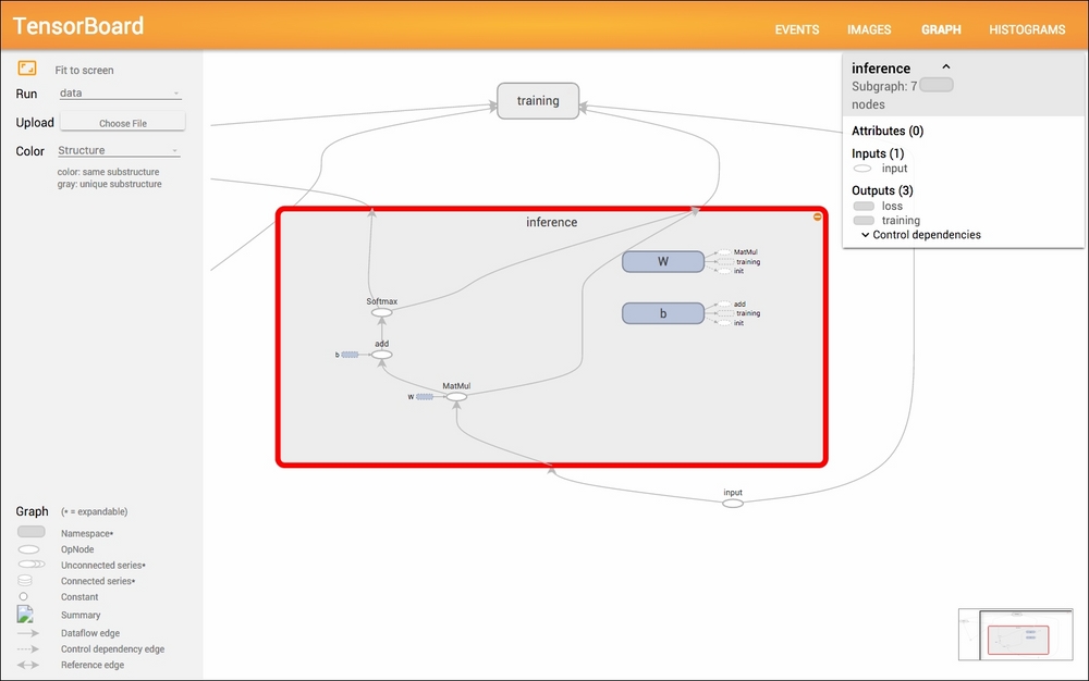
Now let's look inside the code. To enable visualization, you need to wrap the whole area with the scope: with tf.Graph().as_default(). By adding this scope, all the variables declared in the scope will be displayed in the graph. The displayed name can be set by including the name label as follows:

x_placeholder = tf.placeholder("float", [None, 784], name="input")
label_placeholder = tf.placeholder("float", [None, 10], name="label")

Defining other scopes will create nodes in the graph and this is where the division, inference(), loss(), and training() reveal their real values. You can define the respective scope without losing any readability:

def inference(x_placeholder):
    with tf.name_scope('inference') as scope:
        W = tf.Variable(tf.zeros([784, 10]), name="W")
        b = tf.Variable(tf.zeros([10]), name="b")

        y = tf.nn.softmax(tf.matmul(x_placeholder, W) + b)

    return y

def loss(y, label_placeholder):
    with tf.name_scope('loss') as scope:
        cross_entropy = - tf.reduce_sum(label_placeholder * tf.log(y))

        tf.scalar_summary("Cross Entropy", cross_entropy)

    return cross_entropy

def training(loss):
    with tf.name_scope('training') as scope:
        train_step = tf.train.GradientDescentOptimizer(0.01).minimize(loss)

    return train_step

tf.scalar_summary() in loss() makes the variable show up in the EVENTS menu. To enable visualization, we need the following code:

summary_step = tf.merge_all_summaries()
init = tf.initialize_all_variables()

summary_writer = tf.train.SummaryWriter('data', graph_def=sess.graph_def)

Then the process of variables can be added with the following code:

summary = sess.run(summary_step, feed_dict=feed_dict)
summary_writer.add_summary(summary, i)

This feature of visualization will be much more useful when we're using more complicated models.