In the previous chapters, you learned quite a lot about deep learning. You should now understand the fundamentals of the concepts, theories, and implementations of deep neural networks. You also learned that you can experiment with deep learning algorithms on various data relatively easily by utilizing a deep learning library. The next step is to examine how deep learning can be applied to a broad range of other fields and how to utilize it for practical applications.
Therefore, in this chapter, we'll first see how deep learning is actually applied. Here, you will see that the actual cases where deep learning is utilized are still very few. But why aren't there many cases even though it is such an innovative method? What is the problem? Later on, we'll think about the reasons. Furthermore, going forward we will also consider which fields we can apply deep learning to and will have the chance to apply deep learning and all the related areas of artificial intelligence.
The topics covered in this chapter include:
- Image recognition, natural language processing, and the neural networks models and algorithms related to them
- The difficulties of turning deep learning models into practical applications
- The possible fields where deep learning can be applied, and ideas on how to approach these fields
We'll explore the potential of this big AI boom, which will lead to ideas and hints that you can utilize in deep learning for your research, business, and many sorts of activities.
We often hear that research for deep learning has always been ongoing and that's a fact. Many corporations, especially large tech companies such as Google, Facebook, Microsoft, and IBM, invest huge amounts of money into the research of deep learning, and we frequently hear news that some corporation has bought these research groups. However, as we look through, deep learning itself has various types of algorithms, and fields where these algorithms can be applied. Even so, it is a fact that is it not widely known which fields deep learning is utilized in or can be used in. Since the word "AI" is so broadly used, people can't properly understand which technology is used for which product. Hence, in this section, we will go through the fields where people have been trying to adopt deep learning actively for practical applications.
The field in which deep learning is most frequently incorporated is image recognition. It was Prof. Hinton and his team's invention that led to the term "deep learning." Their algorithm recorded the lowest error rates ever in an image recognition competition. The continuous research done to improve the algorithm led to even better results. Now, image recognition utilizing deep learning has gradually been adopted not only for studies, but also for practical applications and products. For example, Google utilizes deep learning to auto-generate thumbnails for YouTube or auto-tag and search photos in Google Photos. Like these popular products, deep learning is mainly applied to image tagging or categorizing and, for example, in the field of robotics, it is used for robots to specify things around them.
The reason why we can support these products and this industry is because deep learning is more suited to image processing, and this is because it can achieve higher precision rates than applications in any other field. Only because the precision and recall rate of image recognition is so high does it mean this industry has broad potential. An error rate of MNIST image classification is recorded at 0.21 percent with a deep learning algorithm (http://cs.nyu.edu/~wanli/dropc/), and this rate can be no lower than the record for a human (http://arxiv.org/pdf/0710.2231v1.pdf). In other words, if you narrow it down to just image recognition, it's nothing more than the fact that a machine may overcome a human. Why does only image recognition get such high precision while other fields need far more improvement in their methods?
One of the reasons is that the structure of feature extractions in deep learning is well suited for image data. In deep neural networks, many layers are stacked and features are extracted from training data step by step at each layer. Also, it can be said that image data is featured as a layered structure. When you look at images, you will unconsciously catch brief features first and then look into a more detailed feature. Therefore, the inherent property of deep learning feature extraction is similar to how an image is perceived and hence we can get an accurate realization of the features. Although image recognition with deep learning still needs more improvements, especially of how machines can understand images and their contents, obtaining high precision by just adopting deep learning to sample image data without preprocessing obviously means that deep learning and image data are a good match.
The other reason is that people have been working to improve algorithms slowly but steadily. For example, in deep learning algorithms, CNN, which can get the best precision for image recognition, has been improved every time it faces difficulties/tasks. Local receptive fields substituted with kernels of convolutional layers were introduced to avoid networks becoming too dense. Also, downsampling methods such as max-pooling were invented to avoid the overreaction of networks towards a gap of image location. This was originally generated from a trial and error process on how to recognize handwritten letters written in a certain frame such as a postal code. As such, there are many cases where a new approach is sought to adapt neural networks algorithms for practical applications. A complicated model, CNN is also built based on these accumulated yet steady improvements. While we don't need feature engineering with deep learning, we still need to consider an appropriate approach to solve specific problems, that is, we can't build omnipotent models, and this is known as the No Free Lunch Theorem (NFLT) for optimization.
In the image recognition field, the classification accuracy that can be achieved by deep learning is extremely high, and it is actually beginning to be used for practical applications. However, there should be more fields where deep learning can be applied. Images have a close connection to many industries. In the future, there will be many cases and many more industries that utilize deep learning. In this book, let's think about what industries we can apply image recognition to, considering the emergence of deep learning in the next sections.
The second most active field, after image recognition, where the research of deep learning has progressed is natural language processing (NLP). The research in this field might become the most active going forward. With regard to image recognition, the prediction precision we could obtain almost reaches the ceiling, as it can perform even better classification than a human could. On the other hand, in NLP, it is true that the performance of a model gets a lot better thanks to deep learning, but it is also a fact that there are many tasks that still need to be solved.
For some products and practical applications, deep learning has already been applied. For example, NLP based on deep learning is applied to Google's voice search or voice recognition and Google translation. Also, IBM Watson, the cognitive computing system that understands and learns natural language and supports human decision-making, extracts keywords and entities from tons of documents, and has functions to label documents. And these functions are open to the public as the Watson API and anyone can utilize it without constraints.
As you can see from the preceding examples, NLP itself has a broad and varied range of types. In terms of fundamental techniques, we have the classification of sentence contents, the classification of words, and the specification of word meanings. Furthermore, languages such as Chinese or Japanese that don't leave a space between words require morphological analysis, which is also another technique available in NLP.
NLP contains a lot of things that need to be researched, therefore it needs to clarify what its purpose is, what its problems are, and how these problems can be solved. What model is the best to use and how to get good precision properly are topics that should be examined cautiously. As for image recognition, the CNN method was invented by solving tasks that were faced. Now, let's consider what approach we can think of and what the difficulties will be respectively for neural networks and NLP. Understanding past trial and error processes will be useful for research and applications going forward.
The fundamental problem of NLP is "to predict the next word given a specific word or words". The problem is too simple, however; if you try to solve it with neural networks, then you will soon face several difficulties because documents or sentences as sample data using NLP have the following features:
- The length of each sentence is not fixed but variable, and the number of words is astronomical
- There can be unforeseen problems such as misspelled words, acronyms, and so on
- Sentences are sequential data, and so contain temporal information
Why can these features pose a problem? Remember the model structure of general neural networks. For training and testing with neural networks, the number of neurons in each layer including the input layer needs to be fixed in advance and the networks need to be the same size for all the sample data. In the meantime, the length of the input data is not fixed and can vary a lot. This means that sample data cannot be applied to the model, at least as it is. Classification or generation by neural networks cannot be done without adding/amending something to this data.
We have to fix the length of input data, and one approach to handle this issue is a method that divides a sentence into a chunk of certain words from the beginning in order. This method is called N-gram. Here, N represents the size of each item, and an N-gram of size 1 is called a unigram, size 2 is a bigram, and size 3 is a trigram. When the size is larger, then it is simply called with the value of N, such as four-gram, five-gram, and so on.
Let's look at how N-gram works with NLP. The goal here is to calculate the probability of a word ![]() given some history
given some history ![]() ;
;![]() . We'll represent a sequence of
. We'll represent a sequence of ![]() words as
words as ![]() . Then, the probability we want to compute is
. Then, the probability we want to compute is ![]() , and by applying the chain rule of probability to this term, we get:
, and by applying the chain rule of probability to this term, we get:

It might look at first glance like these conditional probabilities help us, but actually they don't because we have no way of calculating the exact probability of a word following a long sequence of preceding words, ![]() . Since the structure of a sentence is very flexible, we can't simply utilize sample documents and a corpus to estimate the probability. This is where N-gram works. Actually, we have two approaches to solve this problem: the original N-gram model and the neural networks model based on N-gram. We'll look at the first one to fully understand how the fields of NLP have developed before we dig into neural networks.
. Since the structure of a sentence is very flexible, we can't simply utilize sample documents and a corpus to estimate the probability. This is where N-gram works. Actually, we have two approaches to solve this problem: the original N-gram model and the neural networks model based on N-gram. We'll look at the first one to fully understand how the fields of NLP have developed before we dig into neural networks.
With N-gram, we don't compute the probability of a word given its whole history, but approximate the history with the last N words. For example, the bigram model approximates the probability of a word just by the conditional probability of the preceding word, ![]() , and so follows the equation:
, and so follows the equation:

Similarly, we can generalize and expand the equation for N-gram. In this case, the probability of a word can be represented as follows:
We get the following equation:

Just bear in mind that these approximations with N-gram are based on the probabilistic model called the Markov model, where the probability of a word depends only on the previous word.
Now what we need to do is estimate these N-gram probabilities, but how do we estimate them? One simple way of doing this is called the maximum likelihood estimation (MLE). This method estimates the probabilities by taking counts from a corpus and normalizing them. So when we think of a bigram as an example, we get:

In the preceding formula, ![]() denotes the counts of a word or a sequence of words. Since the denominator, that is, the sum of all bigram counts starting with a word,
denotes the counts of a word or a sequence of words. Since the denominator, that is, the sum of all bigram counts starting with a word, ![]() is equal to the unigram count of
is equal to the unigram count of ![]() , the preceding equation can be described as follows:
, the preceding equation can be described as follows:

Accordingly, we can generalize MLE for N-gram as well:

Although this is a fundamental approach of NLP with N-gram, we now know how to compute N-gram probabilities.
In contrast to this approach, the neural network models predict the conditional probability of a word ![]() given a specific history,
given a specific history, ![]() ;
; ![]() . One of the models of NLP is called the Neural
Network Language Model (NLMM) (http://www.jmlr.org/papers/volume3/bengio03a/bengio03a.pdf), and it can be illustrated as follows:
. One of the models of NLP is called the Neural
Network Language Model (NLMM) (http://www.jmlr.org/papers/volume3/bengio03a/bengio03a.pdf), and it can be illustrated as follows:
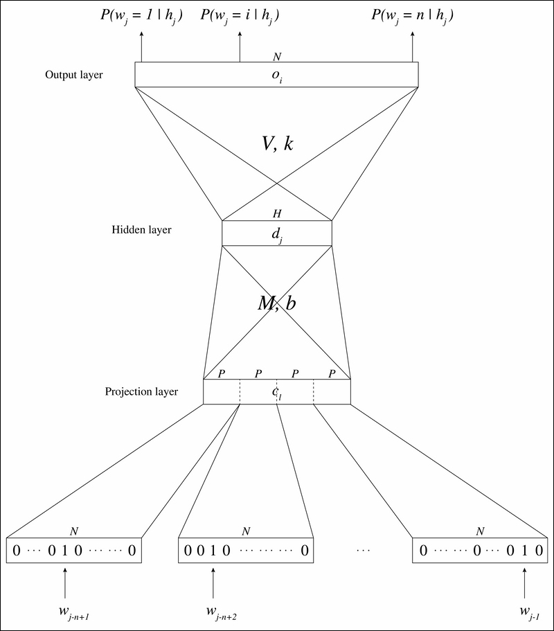
Here, ![]() is the size of the vocabulary, and each word in the vocabulary is an N-dimensional vector where only the index of the word is set to 1 and all the other indices to 0. This method of representation is called 1-of-N coding. The inputs of NLMM are the indices of the
is the size of the vocabulary, and each word in the vocabulary is an N-dimensional vector where only the index of the word is set to 1 and all the other indices to 0. This method of representation is called 1-of-N coding. The inputs of NLMM are the indices of the ![]() previous words
previous words ![]() (so they are n-grams). Since the size N is typically within the range of 5,000 to 200,000, input vectors of NLMM are very sparse. Then, each word is mapped to the projection layer, for continuous space representation. This linear projection (activation) from a discrete to a continuous space is basically a look-up table with
(so they are n-grams). Since the size N is typically within the range of 5,000 to 200,000, input vectors of NLMM are very sparse. Then, each word is mapped to the projection layer, for continuous space representation. This linear projection (activation) from a discrete to a continuous space is basically a look-up table with ![]() entries, where
entries, where ![]() denotes the feature dimension. The projection matrix is shared for the different word positions in the context, and activates the word vectors to projection layer units
denotes the feature dimension. The projection matrix is shared for the different word positions in the context, and activates the word vectors to projection layer units ![]() with
with ![]() . After the projection comes the hidden layer. Since the projection layer is in the continuous space, the model structure is just the same as the other neural networks from here. So, the activation can be represented as follows:
. After the projection comes the hidden layer. Since the projection layer is in the continuous space, the model structure is just the same as the other neural networks from here. So, the activation can be represented as follows:

Here, ![]() denotes the activation function,
denotes the activation function, ![]() the weights between the projection layer and the hidden layer, and
the weights between the projection layer and the hidden layer, and ![]() the biases of the hidden layer. Accordingly, we can get the output units as follows:
the biases of the hidden layer. Accordingly, we can get the output units as follows:
Here, ![]() denotes the weights between the hidden layer and the output layer, and
denotes the weights between the hidden layer and the output layer, and ![]() denotes the biases of the output layer. The probability of a word i given a specific history
denotes the biases of the output layer. The probability of a word i given a specific history ![]() can then be calculated using the softmax function:
can then be calculated using the softmax function:

As you can see, in NNLM, the model predicts the probability of all the words at the same time. Since the model is now described with the standard neural network, we can train the model using the standard backpropagation algorithm.
NNLM is one approach of NLP using neural networks with N-gram. Though NNLM solves the problem of how to fix the number of inputs, the best N can only be found by trial and error, and it is the most difficult part of the whole model building process. In addition, we have to make sure that we don't put too much weight on the temporal information of the inputs here.
Neural networks with N-gram may work with certain cases, but contain some issues, such as what n-grams would return the best results, and do n-grams, the inputs of the model, still have a context? These are the problems not only of NLP, but of all the other fields that have time sequential data such as precipitation, stock prices, yearly crop of potatoes, movies, and so on. Since we have such a massive amount of this data in the real world, we can't ignore the potential issue. But then, how would it be possible to let neural networks be trained with time sequential data?
One of the neural network models that is able to preserve the context of data within networks is recurrent neural network (RNN), the model that actively studies the evolution of deep learning algorithms. The following is a very simple graphical model of RNN:

The difference between standard neural networks is that RNN has connections between hidden layers with respect to time. The input at time ![]() is activated in the hidden layer at time
is activated in the hidden layer at time ![]() , preserved in the hidden layer, and then propagated to the hidden layer at time
, preserved in the hidden layer, and then propagated to the hidden layer at time ![]() with the input at time
with the input at time ![]() . This enables the networks to contain the states of past data and reflect them. You might think that RNN is rather a dynamic model, but if you unfold the model at each time step, you can see that RNN is a static model:
. This enables the networks to contain the states of past data and reflect them. You might think that RNN is rather a dynamic model, but if you unfold the model at each time step, you can see that RNN is a static model:

Since the model structure at each time step is the same as in general neural networks, you can train this model using the backpropagation algorithm. However, you need to consider time relevance when training, and there is a technique called Backpropagation through Time (BPTT) to handle this. In BPTT, the errors and gradients of the parameter are backpropagated to the layers of the past:

Thus, RNN can preserve contexts within the model. Theoretically, the network at each time step should consider the whole sequence up to then, but practically, time windows with a certain length are often applied to the model to make the calculation less complicated or to prevent the vanishing gradient problem and the exploding gradient problem. BPTT has enabled training among layers and this is why RNN is often considered to be one of the deep neural networks. We also have algorithms of deep RNN such as stacked RNN where hidden layers are stacked.
RNN has been adapted for NLP, and is actually one of the most successful models in this field. The original model optimized for NLP is called the recurrent neural network language model (RNNLM), introduced by Mikolov et al. (http://www.fit.vutbr.cz/research/groups/speech/publi/2010/mikolov_interspeech2010_IS100722.pdf). The model architecture can be illustrated as follows:

The network has three layers: an input layer ![]() , a hidden layer
, a hidden layer ![]() , and an output layer
, and an output layer ![]() . The hidden layer is also often called the context layer or the state layer. The value of each layer with respect to the time
. The hidden layer is also often called the context layer or the state layer. The value of each layer with respect to the time ![]() can be represented as follows:
can be represented as follows:

Here, ![]() denotes the sigmoid function, and
denotes the sigmoid function, and ![]() the softmax function. Since the input layer contains the state layer at time
the softmax function. Since the input layer contains the state layer at time ![]() , it can reflect the whole context to the network. The model architecture implies that RNNLM can look up much broader contexts than feed-forward NNLM, in which the length of the context is constrained to N (-gram).
, it can reflect the whole context to the network. The model architecture implies that RNNLM can look up much broader contexts than feed-forward NNLM, in which the length of the context is constrained to N (-gram).
The whole time and the entire context should be considered while training RNN, but as mentioned previously, we often truncate the time length because BPTT requires a lot of calculations and often causes the gradient vanishing/exploding problem when learning long-term dependencies, hence the algorithm is often called truncated BPTT. If we unfold RNNLM with respect to time, the model can be illustrated as follows (in the figure, the unfolded time ![]() ):
):

Here ![]() is the label vector of the output. Then, the error vector of the output can be represented as follows:
is the label vector of the output. Then, the error vector of the output can be represented as follows:
We get the following equation:
Here ![]() is the unfolding time:
is the unfolding time:
The preceding image is the derivative of the activation function of the hidden layer. Since we use the sigmoid function here, we get the preceding equation. Then, we can get the error of the past as follows:
With these equations, we can now update the weight matrices of the model:

Here, ![]() is the learning rate. What is interesting in RNNLM is that each vector in the matrix shows the difference between words after training. This is because
is the learning rate. What is interesting in RNNLM is that each vector in the matrix shows the difference between words after training. This is because ![]() is the matrix that maps each word to a latent space, so after the training, mapped word vectors contain the meaning of the words. For example, the vector calculation of "king" – "man" + "woman" would return "queen". DL4J supports RNN, so you can easily implement this model with the library.
is the matrix that maps each word to a latent space, so after the training, mapped word vectors contain the meaning of the words. For example, the vector calculation of "king" – "man" + "woman" would return "queen". DL4J supports RNN, so you can easily implement this model with the library.
Training with the standard RNN requires the truncated BPTT. You might well doubt then that BPTT can really train the model enough to reflect the whole context, and this is very true. This is why a special kind of RNN, the long short term memory (LSTM) network, was introduced to solve the long-term dependency problem. LSTM is rather intimidating, but let's briefly explore the concept of LSTM.
To begin with, we have to think about how we can store and tell past information in the network. While the gradient exploding problem can be mitigated simply by setting a ceiling to the connection, the gradient vanishing problem still needs to be deeply considered. One possible approach is to introduce a unit that permanently preserves the value of its inputs and its gradient. So, when you look at a unit in the hidden layer of standard neural networks, it is simply described as follows:

There's nothing special here. Then, by adding a unit below to the network, the network can now memorize the past information within the neuron. The neuron added here has linear activation and its value is often set to 1. This neuron, or cell, is called constant error carousel (CEC) because the error stays in the neuron like a carousel and won't vanish. CEC works as a storage cell and stores past inputs. This solves the gradient vanishing problem, but raises another problem. Since all data propagated through is stocked in the neuron, it probably stores noise data as well:

This problem can be broken down into two problems: input weight conflicts and output weight conflicts. The key idea of input weight conflicts is to keep certain information within the network until it's necessary; the neuron is to be activated only when the relevant information comes, but is not to be activated otherwise. Similarly, output weight conflicts can occur in all types of neural networks; the value of neurons is to be propagated only when necessary, and not to be propagated otherwise. We can't solve these problems as long as the connection between neurons is represented with the weight of the network. Therefore, another method or technique of representation is required that controls the propagation of inputs and outputs. But how do we do this? The answer is putting units that act like "gates" before and behind the CEC, and these are called input gate and output gate, respectively. The graphical model of the gate can be described as follows:

Ideally, the gate should return the discrete value of 0 or 1 corresponding to the input, 0 when the gate is closed and 1 when open, because it is a gate, but programmatically, the gate is set to return the value in the range of 0 to 1 so that it can be well trained with BPTT.
It may seem like we can now put and fetch exact information at an exact time, yet another problem still remains. With just two gates, the input gate and output gate, memories stored in the CEC can't be refreshed easily in a few steps. Therefore, we need an additional gate that dynamically changes the value of the CEC. To do this, we add a forget gate to the architecture to control when the memory should be erased. The value preserved in the CEC is overridden with a new memory when the value of the gate takes a 0 or close to it. With these three gates, a unit can now memorize information or contexts of the past, and so it is called an LSTM block or an LSTM memory block because it is more of a block than a single neuron. The following is a figure that represents an LSTM block:

The standard LSTM structure was fully explained previously, but there's a technique to get better performance from it, which we'll explain now. Each gate receives connections from the input units and the outputs of all the units in LSTM, but there is no direct connection from the CEC. This means we can't see the true hidden state of the network because the output of a block depends so much on the output gate; as long as the output gate is closed, none of the gates can access the CEC and it is devoid of essential information, which may debase the performance of LSTM. One simple yet effective solution is to add connections from the CEC to the gates in a block. These are called peephole connections, and act as standard weighted connections except that no errors are backpropagated from the gates through the peephole connections. The peephole connections let all gates assume the hidden state even when the output gate is closed. You've learned a lot of terms now, but as a result, the basic architecture of the whole connection can be described as follows:
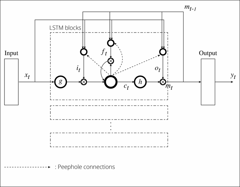
For simplicity, a single LSTM block is described in the figure. You might be daunted because the preceding model is very intricate. However, when you look at the model step by step, you can understand how an LSTM network has figured out how to overcome difficulties in NLP. Given an input sequence ![]() , each network unit can be calculated as follows:
, each network unit can be calculated as follows:

In the preceding formulas, ![]() is the matrix of weights from the input gate to the input,
is the matrix of weights from the input gate to the input, ![]() is the one from the forget gate to the input, and
is the one from the forget gate to the input, and ![]() is the one from the output gate to the input.
is the one from the output gate to the input. ![]() is the weight matrix from the cell to the input,
is the weight matrix from the cell to the input, ![]() is the one from the cell to the LSTM output, and
is the one from the cell to the LSTM output, and ![]() is the one from the output to the LSTM output.
is the one from the output to the LSTM output. ![]() ,
, ![]() , and
, and ![]() are diagonal weight matrices for peephole connections. The
are diagonal weight matrices for peephole connections. The ![]() terms denote the bias vectors,
terms denote the bias vectors, ![]() is the input gate bias vector,
is the input gate bias vector, ![]() is the forget gate bias vector,
is the forget gate bias vector, ![]() is the output gate bias vector,
is the output gate bias vector, ![]() is the CEC cell bias vector, and
is the CEC cell bias vector, and ![]() is the output bias vector. Here,
is the output bias vector. Here, ![]() and
and ![]() are activation functions of the cell input and cell output.
are activation functions of the cell input and cell output. ![]() denotes the sigmoid function, and
denotes the sigmoid function, and ![]() the softmax function.
the softmax function. ![]() is the element-wise product of the vectors.
is the element-wise product of the vectors.
We won't follow the further math equations in this book because they become too complicated just by applying BPTT, but you can try LSTM with DL4J as well as RNN. As CNN was developed within the field of image recognition, RNN and LSTM have been developed to resolve the issues of NLP that arise one by one. While both algorithms are just one approach to get a better performance using NLP and still need to be improved, since we are living beings that communicate using languages, the development of NLP will certainly lead to technological innovations. For applications of LSTM, you can reference Sequence to Sequence Learning with Neural Networks (Sutskever et al., http://arxiv.org/pdf/1409.3215v3.pdf), and for more recent algorithms, you can reference Grid Long Short-Term Memory (Kalchbrenner et al., http://arxiv.org/pdf/1507.01526v1.pdf) and Show, Attend and Tell: Neural Image Caption Generation with Visual Attention (Xu et al., http://arxiv.org/pdf/1502.03044v2.pdf).