
5
C H A P T E R 2
Deep Learning
Machine learning is a powerful tool in AI, where rather than engineer an algorithm to com-
plete a task, the designer can provide the algorithm with examples (i.e., training data) and the
algorithm learns to solve the task on its own. Given enough training data, machine learning
algorithms can optimize their solution to outperform traditional programming methods. Ar-
tificial neural networks are a promising tool for machine learning methods, and have gained
significant attention since the discovery of techniques for training larger multilayer neural net-
works, called deep neural networks. is class of techniques utilizing deep neural networks for
machine learning are referred to as deep learning. Deep learning has been developing rapidly in
recent years and has shown great promise in fields such as computer vision [24], speech recog-
nition [25], and language processing [26]. e aim of this chapter is to provide the reader with
a brief background on neural networks and deep learning methods which are discussed in the
later sections.
Artificial
Intelligence
Machine
Learning
Deep
Learning
Figure 2.1: Deep learning is a subset of machine learning techniques.
2.1 NEURAL NETWORK ARCHITECTURES
e structure of artificial neural networks is inspired by the neural structure of the human brain,
with layers of interconnected neurons transferring information. Figure 2.2 illustrates a simple

6 2. DEEP LEARNING
Input Layer Hidden Layer Output Layer
Figure 2.2: Feedforward neural network.
feedforward neural network. e first layer (on the left) is the input layer, with each neuron
representing an input to the neural network. e second layer is the hidden layer. Although in
the neural network shown in Fig. 2.2 there is only one hidden layer, this number can vary. e
final layer is the output layer, with each neuron representing an output from the neural network.
e neurons send their values to neurons in the next layer. Typically, each neuron is connected
to all neurons in the next layer. is is called a fully connected neural network. Each connection
also has a weight, which multiplies the input to the neuron in the next layer. erefore, the input
at the next layer is a weighted summation of the outputs of the previous layer. e weights of
these connections are changed over time as the neural network learns. e neural network tunes
these weights over the training process to optimize its performance at a given task. Generally, a
loss function is used as a measure of the network error, and network weights are updated such
that the loss is minimized during training.
e hidden neurons also normalize their output by applying an activation function to its
input, such as a Rectified Linear Unit (ReLU) or a sigmoid function. e activation function
is helpful as it introduces some nonlinearity in the neural network. Consider a case of a neural
network with no nonlinearities, since the output of each layer is a linear function, and a sum
of linear functions is still a linear function, the relationship between the input and the network
output could be described by the function F .x/ D mx. To update the weights using gradient
descent, the gradient of this function would be calculated as m. erefore the gradient is not a
function of the inputs x. Moreover, in the case of linear activations, there is no benefit in making
the network deeper as the function F .x/ D mx can always be estimated by a neural network
with a single hidden layer. However, by using nonlinear activation functions, we can make the
networks deeper by introducing more hidden layers and enabling the networks to model more

2.1. NEURAL NETWORK ARCHITECTURES 7
complex relationships. A set of nonlinear activation functions commonly used in deep neural
networks is illustrated in Fig. 2.3.
Sigmoid
1
1 + e
-x
Tanh
tanh(x)
ReLU
max(0,x)
Leaky ReLU
max(0.1x,x)
Softplus
ln(1 + e
x
)
1
0
-10 0 10
-10 0 10
-10 0 10
-10 0 10
-10 0 10
10
0
10
0
10
0
1
-1
0
Figure 2.3: Common activation functions in neural networks.
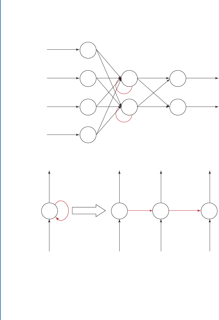
e second class of neural network architectures commonly used are the Recurrent Neu-
ral Networks (RNNs). RNNs provide the neural network with temporal context. As shown in
Fig. 2.4, they are essentially feedforward neural networks, but with the outputs of neurons from
the previous time step as an additional input into the network. is allows the network to re-
member previous inputs and outputs, providing it with memory of previous states and actions.
is is useful in domains where the inputs and outputs are dependent on the inputs and out-
puts of previous time steps. e downside of RNNs is the increased difficulty in training the
network [46–50]. Commonly used recurrent networks include the Long Short-Term Memory
(LSTM) [51] and Gated Recurrent Unit (GRU) [52].
Convolutional neural networks (CNNs) are used for tasks where spatial context is re-
quired, such as image processing tasks. e main types of layers utilized in CNNs are the input,
convolution, pooling, ReLU, and fully connected layers. A typical CNN structure is shown in
Fig. 2.5. e input layer is typically a three-dimensional input, consisting of the raw pixel values
of the image and the RGB color channel values. e convolutional layers are used to compute
the dot product of the convolution filter and a local region of the previous layer. e convolution
8 2. DEEP LEARNING
Input Layer Hidden Layer Output Layer
Unfold in time
h
y
x
y
t-1
x
t-1
y
t+1
x
t+1
y
t
w
t-1
w
t
x
t
w
h
t-1
h
t+1
h
t
(a) Overall RNN architecture
(b) A hidden neuron in an RNN unfolded in time
Figure 2.4: Recurrent neural network, where the red arrows represent temporal connections.
..................Content has been hidden....................
You can't read the all page of ebook, please click here login for view all page.