
Model Comparison and Hierarchical Modeling
The magazine model comparison game
Leaves all of us wishing that we looked like them.
But they have mere fantasy's bogus appeal,
' Cause none obeys fact or respects what is real.1
There are situations in which different models compete to describe the same set of data. In one classic example, the data consist of the apparent positions of the planets and sun against the background stars, during the course of many months. Are these data best described by an earth-centric model or by a solar-centric model? In other words, how should we allocate credibility across the models?
As was emphasized in Chapter 2 (specifically Section 2.1 and following), Bayesian inference is reallocation of credibility over possibilities. In model comparison, the focal possibilities are the models, and Bayesian model comparison reallocates credibility across the models, given the data. In this chapter, we explore examples and methods of Bayesian inference about the relative credibilities of models. We will see that Bayesian model comparison is really just a case of Bayesian parameter estimation applied to a hierarchical model in which the top-level parameter is an index for the models. A central technical point is that a “model” consists of both its likelihood function and prior distribution, and model comparison can be extremely sensitive to the choice of prior, even if the prior is vague, unlike continuous parameter estimation within models.
10.1 General formula and the bayes factor
In this section, we will consider model comparison in a general, abstract way. This will establish a framework and terminology for the examples that follow. If this abstract treatment does not make complete sense to you on a first reading, do not despair, because simple examples quickly follow that illustrate the ideas.
Recall the generic notation we have been using, in which data are denoted as D or y, and the parameters of a model are denoted θ. The likelihood function is denoted p(y|θ), and the prior distribution is denoted p(θ). We are now going to expand that notation so we can make reference to different models. We will include a new indexical parameter m that has value m = 1 for model 1, m = 2 for model 2, and so on. Then the likelihood function for model m is denoted pm(y|θm, m) and the prior is denoted pm(θm|m). Notice that the parameter is given a subscript because each model might involve different parameters. Notice also that the probability density is given a subscript, because different models might involve different distributional forms.
Each model can be given a prior probability, p(m). Then we can think of the whole system of models as a large joint parameter space spanning θ1, θ2, …, and m. Notice the joint space includes the indexical parameter m. Then, on this joint space, Bayes' rule becomes
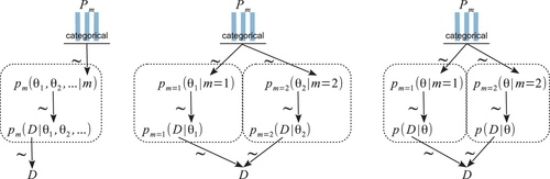
(As usual in Bayes' rule, the variables in the numerator refer to specific values, and the variables in the denominator take on all possible values for the integral or summation.) Notice the key change in going from Equation 10.1 to Equation 10.2 was converting the numerator from an expression about the joint parameter space to an expression of dependencies among parameters. Thus, p(D|θ1, θ2,…,m) p(θ1, θ2,…, m) became Πmpm (D|θm, m) pm(θm|m) p(m). The factoring of the likelihood-times-prior into a chain of dependencies is the hallmark of a hierarchical model.
A hierarchical diagram illustrating these relations appears in Figure 10.1. The left panel shows the general, joint parameter space across all the models, as expressed in Equation 10.1. The middle panel shows the factorization into model subspaces, as expressed in Equation 10.2. The middle panel is meant to emphasize that each submodel has its own parameters and distributions, suggested by the dashed boxes, but the submodels are under a higher-level indexical parameter. The prior on the model index, p(m), is depicted as a bar graph over candidate indexical values m = 1,2,…. (just as the graphical icon for a Bernoulli distribution includes bars over candidate values of y = 0,1).
The aim of this discussion has been to show that this situation is just like any other application of Bayes' rule, but with specific dependencies among parameters, and with the top-level parameter having a discrete, indexical value. Bayesian inference reallocates credibility across the values of the parameters, simultaneously across values of the indexical parameter and across values of the parameters within the component models.
We can also consider Bayes' rule applied to the model index alone, that is, marginalized across the parameters within the component models. This framing is useful when we want to know the relative credibilities of models overall. Bayes' rule says that the posterior probability of model m is 2
where the probability of the data, given the model m, is, by definition, the probability of the data within that model marginalized across all possible parameter values:
Thus, to get from the prior probability of a model, p(m), to its posterior probability, p(m| D), we must multiply by the probability of the data given that model, p(D|m). Notice that the probability of the data for a model, p(D|m), is computed by marginalizing across the prior distribution of the parameters in the model, pm (θm|m). This role of the prior distribution in p(D|m) is a key point for understanding Bayesian model comparison. It emphasizes that a model is not only the likelihood function, but also includes the prior on its parameters. This fact, that a model refers to both the likelihood and the prior, is explicit in the notation that includes the model index in the likelihood and prior, and is also marked in Figure 10.1 as the dashed lines that enclose the likelihood and prior for each model. As we will see, one consequence is that Bayesian model comparison can be very sensitive to the choice of priors within models, even if those priors are thought to be vague.
Suppose we want to know the relative posterior probabilities of two models. We can write Equation 10.3 once with m = 1 and again with m = 2 and take their ratio to get:
The ratio at the end, underbraced with “ = 1,” equals 1 and can be removed from the equation. The ratio underbraced and marked with “BF” is the Bayes factor for models 1 and 2. The Bayes factor (BF) is the ratio of the probabilities of the data in models 1 and 2. Those probabilities are marginalized across the parameters within each model, as expressed by Equation 10.4. Thus, Equation 10.5 says that the so-called “posterior odds” of two models are the “prior odds” times the Bayes factor. The Bayes factor indicates how much the prior odds change, given the data. One convention for converting the magnitude of the BF to a discrete decision about the models is that there is “substantial” evidence for model m = 1 when the BF exceeds 3.0 and, equivalently, “substantial” evidence for model m = 2 when the BF is less than 1/3 (Jeffreys, 1961; Kass & Raftery, 1995; Wetzels et al., 2011).
10.2 Example: two factories of coins
We will consider a simple, contrived example in order to illustrate the concepts and mechanisms. Suppose we have a coin, embossed with the phrase, “Acme Novelty and Magic Company, Patent Pending.” We know that Acme has two coin factories. One factory generates tail-biased coins, and the other factory generates head-biased coins. The tail-biased factory generates coins with biases distributed around a mode of ω1 = 0.25, with a consistency (or concentration) of κ = 12, so that the biases of coins from the factory are distributed as θ ∼ beta(θ|ω1 (κ − 2) +1, (1 − ω1(κ − 2)+1) = beta(θ|3.5, 8.5). The head-biased factory generates coins with biases distributed around a mode of ω2 = 0.75, again with a consistency of κ = 12, such that the biases of coins from the factory are distributed as θ ∼ beta(θ|ω2 (κ − 2) +1, (1 − ω2 (κ − 2) + 1) = beta(θ|8.5, 3.5).
A diagram representing the two factories is shown in Figure 10.2. The two models are shown within the two dashed boxes. The left dashed box shows the tail-biased model, as suggested by the beta-distributed prior that has its mode at 0.25. The right dashed box shows the head-biased model, as suggested by the beta-distributed prior that has its mode at 0.75. At the top of the diagram is the indexical parameter m, and we want to compute the posterior probabilities of m = 1 and m = 2, given the observed flips of the coin, yi. The diagram in Figure 10.2 is a specific case of the right panel of Figure 10.1, because the likelihood function is the same for both models and only the priors are different.
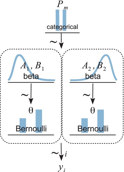
Suppose we flip the coin nine times and get six heads. Given those data, what are the posterior probabilities of the coin coming from the head-biased or tail-biased factories? We will pursue the answer three ways: via formal analysis, grid approximation, and MCMC.
10.2.1 Solution by formal analysis
Both the tail-biased and head-biased models have prior distributions that are beta density functions, and both models use the Bernoulli likelihood function. This is exactly the form of model for which we derived Bayes' rule analytically in Equation 6.8 (p. 132). In that equation, we denoted the data as z, N to indicate z heads in N flips. The derivation showed that if we start with a beta(θ |a, b) prior, we end up with a beta(θ|z + a, N−z+b) posterior. In particular, it was pointed out in Footnote 5 on p. 132 that the denominator of Bayes' rule, that is, the marginal likelihood, is

Equation 10.6 provides an exact formula for the value of p(D|m). Here is a function in R that implements Equation 10.6:
That function works fine for modest values of its arguments, but unfortunately it suffers underflow errors when its arguments get too big. A more robust version converts the formula into logarithms, using the identity that

The logarithmic form of the beta function is built into R as the function lbeta. Therefore, we instead use the following form:
Let's plug in the specific priors and data to compute exactly the posterior probabilities of the two factories. First, consider the tail-biased factory (model index m = 1). For its prior distribution, we know ω1 = 0.25 and κ = 12, hence a1 = 0.25 · 10 + 1 = 3.5 and b1 = (1 − 0.25) · 10 + 1 = 8.5. Then, from Equation 10.6, p(D|m = 1) = p(z, N|m = 1) = B(z + a1, N − z + b1)/B(a1, b1) ≈ 0.000499, which you can verify in R using pD(z = 6,N = 9,a = 3.5,b = 8.5). Next, consider the head-biased factory (model index m = 2). For its prior distribution, we know ω = 0.75 and κ = 12, hence a2 = 0.75·10+1 = 8.5 and b2 = (1−0.75)·10+1 = 3.5. Then, from Equation 10.6, p(D|m = 2) = p(z, N|m = 2) = B(z + a2, N − z + b2)/B(a2, b2) ≈ 0.002339. The Bayes factor is p(D|m = 1)/p(D|m = 2) = 0.000499/0.002339 = 0.213. In other words, if the prior odds for the two factories were 50/50, then the posterior odds are 0.213 against the tail-biased factory, which is to say 4.68 (i.e., 1/0.213) in favor of the head-biased factory.
We can convert the Bayes factor to posterior probabilities, assuming specific prior probabilities, as follows: we start with Equation 10.5 and plug in the values of the Bayes factor and the prior probabilities. Here, we assume that the prior probabilities of the models are p(m = 1) = p(m = 2) = 0.5.
And therefore p(m = 2|D) = 82.4%. (These percentages were computed by retaining more significant digits than were presented in the rounded values above.) In other words, given the data, which showed six heads in nine flips, we reallocated beliefs from a prior head-biased credibility of p(m = 2) = 50% to a posterior head-biased credibility of p(m = 2|D) = 82.4%.
Exercise 10.1 has you explore variations of this scheme. In particular, when the models make very different predictions, which in this case means the factories produce very different biases, then only a small amount of data is needed to strongly prefer one model over the other.
Notice that the model comparison only indicates the relative probabilities of the models. It does not, by itself, provide a posterior distribution on the coin bias. In the above calculations, there was nothing derived for p(θ| D, m). Thus, while we have estimated which factory might have produced the coin, we have not estimated what the bias of the coin might be!
10.2.2 Solution by grid approximation
The analytical solution of the previous section provides an exact answer, but reproducing it with a grid approximation provides additional insights when we visualize the parameter space.
In our current scenario, the model index, m, determines the value of the factory mode, ωm. Therefore, instead of thinking of a discrete indexical parameter m, we can think of the continuous mode parameter ω being allowed only two discrete values by the prior. The overall model has only one other parameter, namely the coin bias θ. We can graph the prior distribution on the ω, θ parameter space as shown in the upper panels of Figure 10.3. Notice that the prior is like two dorsal fins, each having the profile of a beta distribution, with one fin at ω = 0.25 and the other fin at ω = 0.75. These two fins correspond to the two beta distributions shown in Figure 10.2.
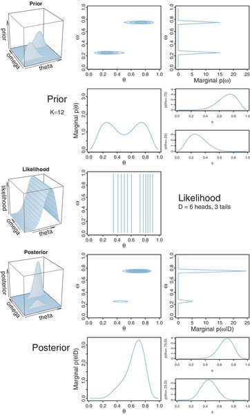
Importantly, notice the top-right panel of Figure 10.3, which shows the marginal prior distribution on ω. You can see that it is two spikes of equal heights, which means that the prior puts equal probability on the two candidate values of ω for the two models. (The absolute scale on p(ω) is irrelevant because it is the probability density for an arbitrary choice of grid approximation.) The two-spike prior on ω represents the discrete prior on the model index, m.
One advantage of the visualization in Figure 10.3 is that we can see both models simultaneously and see the marginal prior distribution on θ when averaging across models. Specifically, the middle panel of the second row shows p(θ),where you can see it is a bimodal distribution. This illustrates that the overall model structure, as a whole, asserts that biases are probability near 0.25 or 0.75.
The likelihood is shown in the middle row of Figure 10.3, again for data consisting of z = 6 heads in N = 9 flips. Notice that the level contours of the likelihood depend only on the value of θ, as they should.
The posterior distribution is shown in the lower two rows of Figure 10.3. The posterior distribution was computed at each point of the ⟨θ, ω⟩ grid by multiplying prior times likelihood, and then normalizing (exactly as done for previous grid approximations such as in Figure 9.2, p. 227).
Notice the marginal posterior distribution on ω, shown in the right panel of the fourth row. You can see that the spike over ω = 0.75 is much taller than the spike over ω = 0.25. In fact, visual inspection suggests that the ratio of the heights is about 5 to 1, which matches the Bayes factor of 4.68 that we computed exactly in the previous section. (As mentioned above, the absolute scale on p(ω) is irrelevant because it is the probability density for an arbitrary choice of grid approximation.) Thus, at the level of model comparison, the grid approximation has duplicated the analytical solution of the previous section. The graphs of the spikes on discrete levels of ω provide a visual representation of model credibilities.
The visualization of the grid approximation provides additional insights, however. In particular, the bottom row of Figure 10.3 shows the posterior distribution of θ within each discrete value of ω, and the marginal distribution of θ across values of ω. If we restrict our attention to the model index alone, we do not see the implications for θ. One way of verbally summarizing the posterior distribution is like this: Given the data, the head-biased factory (with ω = 0.75) is about five times more credible than the tail-biased factory (with ω = 0.25), and the bias of the coin is near θ = 0.7 with uncertainty shown by the oddly-skewed distribution3 in the bottom-middle panel of Figure 10.3.
10.3 Solution by MCMC
For large, complex models, we cannot derive p(D|m) analytically or with grid approximation, and therefore we will approximate the posterior probabilities using MCMC methods. We will consider two approaches. The first approach computes p(D|m) using MCMC for individual models. The second approach puts the models together into a hierarchy as diagrammed in Figure 10.1, and the MCMC process visits different values of the model index proportionally to their posterior probabilities.
10.3.1 Nonhierarchical MCMC computation of each model's marginal likelihood
In this section, we consider how to compute p(D|m) for a single model m. This section is a little heavy on the math, and the method has limited usefulness for complex models, and may be of less immediate value to readers who wish to focus on applications in the latter part of the book. Therefore this section may be skipped on a first reading, without loss of dignity. But you will have less to talk about at parties. The method presented in this section is just one of many; Friel and Wyse (2012) offer a recent review.
To explain how the method works, we first need to establish a basic principle of how to approximate functions on probability distributions: For any function f(θ), the integral of that function, weighted by the probability distribution p(θ), is approximated by the average of the function values at points sampled from the probability distribution. In math:

To understand why that is true, consider discretizing the integral in the left side of Equation 10.7, so that it is approximated as a sum over many small intervals: ∫ dθ f (θ) p(θ) ≈ Σj[Δθ p(θj)]f (θj), where θj is a representative value of θ in the jth interval. The term in brackets, Δθ p(θj), is the probability mass of the small interval around θj. That probability mass is approximated by the relative number of times we happen to get a θ value from that interval when sampling from p(θ). Denote the number of times we get a θ value from the jth interval as nj, and the total number of sampled values as N. With a large sample, notice that nj/N ≈ Δθ p(θj). Then  . In other words, every time we sample a θ value from the jth interval, we add into the summation another iteration of the interval's representative value, f (θj). But there is no need to use the interval's representative value; just use the value of f(θ) at the sampled value of θ, because the sampled θ already is in the jth interval. So the approximation becomes
 ![]() , which is Equation 10.7.
, which is Equation 10.7.
For the goal of model comparison, we want to compute the marginal likelihood for each model, which is p(D) = ∫ dθ p(D|θ) p(θ), where p(θ) is the prior on the parameters in the model. In principle, we could just apply Equation 10.7 directly:

This means that we are getting random values from the prior. But in practice, the prior is very diffuse, and for nearly all of its sampled values, p(D|θ) is nearly zero. Therefore, we might need a ginormous number of samples for the approximation to converge to a stable value.
Instead of sampling from the prior, we will use our MCMC sample from the posterior distribution, in a clever way. First, consider Bayes' rule:
We can rearrange it to get
Now a trick (due to Gelfand & Dey, 1994; summarized by Carlin & Louis, 2009): for any probability density function h(θ), it is the case that it integrates to 1, which expressed mathematically is ∫ dθ h(θ) = 1. We will multiply the rearranged Bayes' rule by 1:

where the last line is simply applying Equation 10.7 to the penultimate line. Now I reveal the magic in the transition from second to third lines of Equation 10.8. The θ in h(θ) varies over the range of the integral, but the θ in p(θ|D)/p(D|θ)p(θ) is a specific value. Therefore, we cannot treat the two θ's as interchangeable without further justification. However, the value of the ratio p(θ|D/p(D|θ)p(θ) is the same value for any value of θ, because the ratio always equals the constant 1/p(D), and therefore we can let the value of θ in p(θ|D)/p(D|θ)p(θ) equal the value of θ in h(θ) as the latter varies. In other words, although the θ in p(θ|D)/p(D|θ)p(θ) began as a single value, it transitioned into being a value that varies along with the θ in h(θ). This magic trick is great entertainment at parties.
All there is yet to do is specify our choice for the function h(θ). It would be good for h(θ) to be similar to p(D|θ) p(θ), so that their ratio, which appears in Equation 10.8, will not get too extremely large or extremely small for different values of θ. If their ratio did get too big or small, that would upset the convergence of the sum as N grows.
When the likelihood function is the Bernoulli distribution, it is reasonable that h(θ) should be a beta distribution with mean and standard deviation corresponding to the mean and standard deviation of the samples from the posterior. The idea is that the posterior will tend to be beta-ish, especially for large-ish data sets, regardless of the shape of the prior, because the Bernoulli likelihood will overwhelm the prior as the amount of data gets large. Because I want h(θ) to be a beta distribution that mimics the posterior distribution, I will set the beta distribution's mean and standard deviation to the mean and standard deviation of the θ values sampled from the posterior. Equation 6.7, p. 131, provides the corresponding shape parameters for the beta distribution. To summarize: We approximate p(D) by using Equation 10.8 with h(θ) being a beta distribution with its a and b values set to imitate the posterior distribution. Note that Equation 10.8 yields the reciprocal of p(D), so we have to invert the result to get p(D) itself.
In general, there might not be strong theoretical motivations to select a particular h(θ) density. No matter. All that's needed is any density that reasonably mimics the posterior. In many cases, this can be achieved by first generating a representative sample of the posterior, and then finding an “off-the-shelf” density that describes it reasonably well. For example, if the parameter is limited to the range [0,1], we might be able to mimic its posterior with a beta density that has the same mean and standard deviation as the sampled posterior, even if we have no reason to believe that the posterior really is exactly a beta distribution. If the parameter is limited to the range [0, +∞),then we might be able to mimic its posterior with a gamma density (see Figure 9.8 , p. 237) that has the same mean and standard deviation as the sampled posterior, even if we have no reason to believe that the posterior really is exactly a gamma distribution.
For complex models with many parameters, it may be difficult to create a suitable h(θ), where θ here represents a vector of many parameters. One approach is to mimic the marginal posterior distribution of each individual parameter, and to let h(θ) be the product of the mimicked marginals. This approach assumes that there are no strong correlations of parameters in the posterior distribution, so that the product of marginals is a good representation of the joint distribution. If there are strong correlations of parameters in the posterior distribution, then this approach may produce summands in Equation 10.8 for which h(θi) is large but p(D|θ)p(θi) is close to zero, and their ratio “explodes.” Even if the mimicry by h(θ) is good, the probability densities of the various terms might get so small that they exceed the precision of the computer. Thus, for complex models, this method might not be tractable. For the simple application here, however, the method works well, as demonstrated in the next section.
10.3.1.1 Implementation with JAGS
We have previously implemented the Bernoulli-beta model in JAGS, as the introductory example in Section 8.2, in the program named Jags-Ydich-Xnom1subj-Mbern Beta.R. We will adapt the program so it uses the priors from the current model comparison, and then use its MCMC output to compute p(D) in R from Equation 10.8.
In the model section of Jags-Ydich-Xnom1subj-MbernBeta.R, change the prior to the appropriate model. For example, for m = 2, which has ω = 0.75 and κ = 12, we simply change the constants in the dbeta prior as follows:
Be sure to save the altered file, perhaps with a different file name than the original. Then generate the MCMC posterior sample with these commands:
Having thereby generated the MCMC chain and put it in a vector named theta, we then compute p(D) by implementing Equation 10.8 in R:
The result is PD= 0.002338 for one JAGS run, which is remarkably close to the value computed from formal analysis. Repeating the above, but with the model statement and formula for oneOverPD using ω = 0.25, yields PD= 0.000499 for one JAGS run, which is also remarkably close to the value computed from formal analysis.
10.3.2 Hierarchical MCMC computation of relative model probability
In this section, we implement the full hierarchical structure depicted by Figure 10.2 (p. 269), in which the top-level parameter is the index across models. The specific example is implemented in the R script Jags-Ydich-Xnom1subj-MbernBetaModel Comp.R. (The program is a script run on its own, not packaged as a function and called from another program, because this example is a specialized demonstration that is unlikely to be used widely with different data sets.)
The data are coded in the usual way, with y being a vector of 0's and 1's. The variable N is the total number of flips. The model of Figure 10.2 (p. 269) can then be expressed in JAGS as follows:
As you read through the model specification (above), note that the Bernoulli likelihood function and beta prior distribution are only specified once, even though they participate in both models. This is merely a coding convenience, not a necessity. In fact, a later section shows a version in which distinct beta distributions are used. Importantly, notice that the value of omega[m] in the beta distribution depends on the model index, m. The next lines in the model specification assign the particular values for omega[1] and omega[2]. At the end of the model specification, the top-level prior on the model index is a categorical distribution, which is denoted dcat in JAGS. The argument of the dcat distribution is a vector of probabilities for each category. JAGS does not allow the vector constants to be defined inside the argument, like this: m ∼ dcat(c(.5,.5)). With the model specified as shown above, the rest of the calls to JAGS are routine.
When evaluating the output, it is important to keep in mind that the sample of theta values is a mixture of values combining cases of m=1 and m=2. At every step in the MCMC chain, JAGS provides representative values of θ and m that are jointly credible, given the data. At any step in the chain, JAGS lands on m = 1 or m = 2 proportionally to each model's posterior probability, and, for whichever value of m is sampled at that step, JAGS produces a credible value of θ for the corresponding ωm. If we plot a histogram of all the theta values, collapsed across model indices, the result looks like the bottom-middle panel of Figure 10.3. But if we want to know the posterior distribution of θ values within each model, we have to separate the steps in the chain for which m = 1 or m = 2. This is trivial to do in R; see the script.
Figure 10.4 shows the prior and posterior distributions of m, θ1, and θ2. The prior was generated from JAGS in the usual way; see Section 8.5 (p. 211). Notice that the prior is as intended, with a 50-50 categorical distribution on the model index, and the appropriate tail-biased and head-biased priors on θ1 and θ2. The lower frame of Figure 10.4 shows the posterior distribution, where it can be seen that the results match those of the analytical solution, the grid approximation, and the one-model-at-a-time MCMC implementation of previous sections.

In particular, the posterior probability of m = 1 is about 18%. This means that during the MCMC random walk, the value m = 1 was visited on only about 18% of the steps. Therefore the histogram of θ1 is based on only 18% of the chain, while the histogram of θ2 is based on the complementary 82% of the chain. If the data were to favor one model over the other very strongly, then the losing model would have very few representative values in the MCMC sample.
10.3.2.1 Using pseudo-priors to reduce autocorrelation
Here we consider an alternative way to specify the model of the previous section, using two distinct beta distributions that generate distinct θm values. This method is more faithful to the diagram in Figure 10.2, and it is also more general because it allows different functional forms for the priors, if wanted. For realistic, complex model comparison, the implementation techniques described in this section are needed (or some other technique altogether, as opposed to the simplification of the previous section).
In this implementation, there are three parameters in the model, namely m, θ1, and θ2. At every step in the MCMC random walk, JAGS generates values of all three parameters that are jointly credible, given the data. However, at any step in the chain, only the θm of the sampled model index m is actually used to describe the data. If, at some step in the chain, the sampled value of m is 1, then θ1 is used to describe the data, while θ2 floats free of the data, constrained only by its prior. If, at another step in the chain, the sampled value of m is 2, then θ2 is used to describe the data, and θ1 is constrained only by its prior.
Let's take a look at this model structure in JAGS, to see how it works. One novel requirement is that we must somehow tells JAGS to use θ1 when m = 1 but to use θ2 when m = 2. We cannot do this with an if statement, as we might use in R, because JAGS is not a procedural language. The JAGS model specification is a “static” declaration of structure, not a sequential script of commands. Therefore, we use the JAGS equals(,) function, which returns TRUE (or 1) if its arguments are equal, and returns FALSE (or 0) if its arguments are not equal. Thus, the JAGS statement
sets theta to the value of theta1 when m equals 1 and sets theta to the value of theta2 when m equals 2.
Below is the complete model specification for JAGS. Notice that theta1 and theta2 have different dbeta priors. The priors are given ω and κ values that match the examples of previous sections.
The model specified above will run in JAGS without any problems in principle. In practice, however, for model structures of this type, the chain for the model index can be highly autocorrelated: The chain will linger in one model for a long time before jumping to the other model. In the very long run, the chain will visit each model proportionally to its posterior probability, but it might take a long time for the visiting proportion to represent the probability accurately and stably. Therefore, we will implement a trick in JAGS to help the chain jump between models more efficiently. The trick uses so-called “pseudopriors” (Carlin & Chib, 1995).
To motivate the use of pseudopriors, we must understand why the chain may have difficulty jumping between models. As was mentioned above, at each step in the chain, JAGS generates values for all three parameters. At a step for which m = 1, then θ1 is used to describe the data, while θ2 floats unconstrained by the data and is sampled randomly from its prior. At a step for which m = 2, then θ2 is used to describe the data, while θ1 floats unconstrained by the data and is sampled randomly from its prior. The problem is that on the next step, when JAGS considers a new random value for m while leaving the other parameter values unchanged, JAGS is choosing between the current value of m, which has a value for θm = current that is credible for the data, and the other value m, which has a value for θm = other from its prior that might be far away from posterior credible values. Because θm = other might be a poor description of the data, the chain rarely jumps to it, instead lingering on the current model.
A solution to this problem is to make the unused, free-floating parameter values remain in their zone of posterior credibility. Recall that parameter values are generated randomly from their prior when not being used to describe data. If we make the prior mimic the posterior when the parameter is not being used to describe data, then the randomly generated value will remain in the credible zone. Of course, when the parameter is being used to describe the data, then we must use its true prior. The prior that is used when the parameter is not describing the data is called the pseudoprior. Thus, when the model index is m = 1, θ1 uses its true prior and θ2 uses its pseudoprior. When the model index is m = 2, then θ2 uses its true prior and θ1 uses its pseudoprior.
To implement pseudopriors in JAGS, we can establish indexed values for the prior constants. Instead of using a single value omega1 for the mode of the prior beta on theta1, we will instead use a mode indexed by the model, omega1[m], which has different values depending on m. Thus, instead of specifying a single prior for theta1 like this,
we will specify a prior that depends on the model index, like this:
In particular, notice that omega1[1] refers to the true prior value because it is the mode for theta1 when m=1, but omega1[2] refers to the pseudo-prior value because it is the mode for theta1 when m=2. The point of the above example is for you to understand the indexing. How to set the constants for the pseudo-priors is explained in the example below.
To show clearly the phenomenon of autocorrelation in the model index, the example will use data and prior constants that are a little different than the previous example. The data consist of z = 17 heads in N = 30 flips. Model 1 has ω1 = 0.10 with κ1 = 20, and model 2 has ω2 = 0.90 with κ2 = 20. The JAGS model specification therefore has true priors specified as follows:
The complete script for this example has file name Jags-Ydich-Xnom1subj-MbernBetaModelCompPseudoPrior.R.
The values for the pseudo-priors are determined as follows:
1. Do an initial run of the analysis with the pseudo-prior set to the true prior. Note the characteristics of the marginal posterior distributions on the parameters.
2. Set the pseudo-prior constants to values that mimic the currently estimated posterior. Run the analysis. Note the characteristics of the marginal posterior distributions on the parameters. Repeat this step if the pseudo-prior distributions are very different from the posterior distributions.
As an example, Figure 10.5 shows an initial run of the analysis, using the true prior for the pseudoprior values. The MCMC chain had 10,000 steps altogether. The top part of the figure shows the convergence diagnostics on the model index. In particular, you can see from the top-right panel that the effective sample size (ESS) of the chain is very small, in this case less than 500. The top-left panel shows that that within each chain the model index lingered at one value for many steps before eventually jumping to the other value.

The lower part of Figure 10.5 shows the posterior distribution on the parameters. Consider the panel in the left column of the penultimate row, which shows θ1 when m = 1. This represents the actual posterior distribution on θ1. Below it, in the bottom-left panel, is θ1 when m = 2. These values of θ1 are not describing the data, because they were generated randomly from the prior when JAGS was instead using θ2 to describe the data. Thus, the lower-left panel shows the prior on θ1, which has its mode very close to the model-specified value of ω1 = 0.10. Notice that the (prior) values of θ1 when m = 2 are not very close to the (posterior) values of θ1 when m = 1. Analogously, the bottom-right panel shows the posterior distribution of θ2 when m = 2, and the panel immediately above it shows the distribution of θ2 when m = 1, which is the prior distribution of θ2 (which has a mode of ω2 = 0.90). Again, notice that the (prior) values of θ2 when m = 1 are not very close to the (posterior) values of θ2 when m = 2.
With an eye on the lower two rows of Figure 10.5, consider the MCMC steps in JAGS. Suppose that at some step it is the case that m = 2, which means we are in the bottom row of Figure 10.5, so θ1 has a value from the bottom-left distribution and θ2 has a value from the bottom-right distribution. Now JAGS considers jumping from m = 2 to m = 1, using its current values of θ1 and θ2. Unfortunately, θ1 is (probably) set to a value that is not among the credible values, and therefore JAGS has little incentive to jump to m = 1. Analogous reasoning applies when m = 1: The present value of θ2 is (probably) not among the credible values, so JAGS is unlikely to jump to m = 2.
Despite the severe autocorrelation in the model index, the initial run has provided an indication of the posterior distributions of θ1 and θ2. We use their characteristics to set their pseudopriors. In particular, the posterior mode of θ1 is near 0.40, so we set omega1[2] <- .40, and the posterior mode of θ2 is near 0.70, so we set omega2[1] <- .70. The κ values were determined by remembering that the concentration parameter increases by N (recall the updating rule for Bernoulli-beta model in Section 6.3). Because the prior κ is 20, and the data have N = 30, the pseudoprior κ is 50, which is specified in the model statement as kappa1[2] <- 50 and kappa2[1] <- 50.
Figure 10.6 shows the results when running the model with the new specification of the pseudopriors. The top-right panel shows that the chain for the model index has virtually no autocorrelation, and the ESS is essentially equal to the total length of the chain. The bottom two rows show the distributions of θ1 and θ2. Notice that the pseudo-priors nicely mimic the actual posteriors.

Because the ESS of the model index is far better than in the initial run, we trust its estimate in this run more than in the initial run. In this second run, with the pseudopriors appropriately set, the posterior probability of m = 2 is very nearly 92%. In the initial run, the estimate was about 89%. While these estimates are not radically different in this case, the example does illustrate what is at stake.
When examining the output of JAGS, it is important to realize that the chain for θm is a mixture of values from the true posterior and the pseudoprior. The values for the true posterior are from those steps in the chain when the model index corresponds to the parameter. Below is an example of R code, from the script Jags-Ydich- Xnom1subj-MbernBetaModelCompPseudoPrior.R, that extracts the relevant steps in the chain. The MCMC output of JAGS is the coda object named codaSamples.
In the above R code, mcmcMat is a matrix with columns named m, theta1 ,and theta2, because those were the monitored variables in the call to JAGS that created the MCMC chain. The vector m contains a sequence of 1's and 2's indicating which model is used at each step. Then mcmcMat[,"theta1"][m==1] consists of the rows of theta1 for which the model index is 1. These are the values of theta1 for the true posterior. Analogously, mcmcMat[,"theta2"][m==2] contains the true posterior values for theta2.
The focus of model comparison is the posterior probability of the model index, m, not the estimates of the parameters in each model. If, however, you are interested in the parameters within each model, then you will want a sufficiently large MCMC sample within each model. In the present example, the chain visited m = 1 in only about 8% of its steps, yielding only about 800 representative values instead of the typically desired 10,000. (The small MCMC sample explains the choppy appearance of the histograms for m = 1.) To increase the number of values, we could simply increase the length of the chain, and wait. In large models with lots of data, however, increasing the chain length might exceed our patience. Instead, we can make JAGS sample more equally between the models by changing the prior on the models to compensate for their relative credibilities. From the initial run using 50-50 priors, we note that p(m = 1|D) ≈ 0.11 and p(m = 2|D) ≈ 0.89. Therefore, in the next run, we set mPriorProb[1] <- .89 and mPriorProb[2] <- .11. The result is that the chain visits the two models about equally often, so we get a better representation of the parameters within each model. This may also provide a better estimate of the relative probabilities of the models, especially if one model is much better than the other.
But, you might ask, if we don't use 50-50 priors, how do we know the posterior probabilities of the models for 50-50 priors? The answer is revealed through the miracle of algebra. Let BF denote the value of the Bayes factor for the models (it is a constant). We know from Equation 10.5, p. 268, that p(m = 1 |D)/p(m = 2|D) = BF · p(m = 1)/p(m = 2). In particular, for 50-50 priors, that equation reduces to p(m = 1 |D)/p(m = 2|D) = BF. Therefore, if we want the posterior odds when the prior odds are 50/50, all we need is BF, which is given by rearranging the general equation: BF =[p(m = 1|D)/p(m = 2|D)]·[p(m = 2)/p(m = 1)].
Another example of model comparison using pseudopriors is presented in Section 12.2.2.1, p. 351. For more information about pseudopriors in transdimensional MCMC, see the tutorial article by Lodewyckx et al. (2011), and the original article by Carlin and Chib (1995), among other useful examples presented by Dellaportas, Forster, and Ntzoufras (2002), Han and Carlin (2001), and Ntzoufras (2002).
10.3.3 Models with different “noise” distributions in JAGS
All of the examples to this point have been cases of the structure in the far right panel of Figure 10.1. In that structure, the probability density function, p(D|θ), is the same for all models. This probability distribution is sometimes called the “noise” distribution because it describes the random variability of the data values around the underlying trend. In more general applications, different models can have different noise distributions. For example, one model might describe the data as log-normal distributed, while another model might describe the data as gamma distributed. The distinct noise distributions are suggested by the middle panel of Figure 10.1, where the likelihood functions have their probability functions subscripted with different indices: p1 (D|θ1, m1) vs p2(D|θ2, m2).
To implement the general structure in JAGS, we would like to tell JAGS to use different probability density functions depending on the value of an indexical parameter. Unfortunately, we cannot use syntax such as y[i] ∼ equals(m,1) *pdf1(param1) + equals(m,2)*pdf2(param2). Instead, we can use the ones trick from Section 8.6.1, p. 214. The general form is shown here:
Notice above that each likelihood function is defined as an explicit formula for its probability density function, abbreviated above as pdf1 or pdf2. Then one of the probability density values, pdf1 or pdf2, is selected for the current MCMC step by using the equals construction. Each likelihood function should be specified in its entirety and both likelihood functions must be scaled by the same constant, C. The prior distributions on the parameters, including the model index, are then set up in JAGS as usual. Of course, the prior distributions on the parameters should use pseudopriors to facilitate efficient sampling of the model index.
10.4 Prediction: Model averaging
In many applications of model comparison, the analyst wants to identify the best model and then base predictions of future data on that single best model, denoted with index b. In this case, predictions of future ![]() are based exclusively on the likelihood function
are based exclusively on the likelihood function ![]() and the posterior distribution pb (θb|D, m = b) of the winning model:
and the posterior distribution pb (θb|D, m = b) of the winning model:
But the full model of the data is actually the complete hierarchical structure that spans all the models being compared, as indicated in Figure 10.1 (p. 267). Therefore, if the hierarchical structure really expresses our prior beliefs, then the most complete prediction of future data takes into account all the models, weighted by their posterior credibilities. In other words, we take a weighted average across the models, with the weights being the posterior probabilities of the models. Instead of conditionalizing on the winning model, we have
This is called model averaging.
The difference between pb(θb|D, m = b) and Σmpm(θm|D, m)p(m|D) is illustrated by the bottom row of Figure 10.3, p. 272. Recall that there were two models of mints that created the coin, with one mint being tail-biased with mode ω = 0.25 and one mint being head-biased with mode ω = 0.75. The two subpanels in the lower-right illustrate the posterior distributions on θ within each model, p(θ|D, ω = 0.25) and p(θ|D, ω = 0.75). The winning model was ω = 0.75, and therefore the predicted value of future data, based on the winning model alone, would use p(θ|D, ω = 0.75). But the overall model included ω = 0.25, and if we use the overall model, then the predicted value of future data should be based on the complete posterior summed across values of ω. The complete posterior distribution, p(θ|D), is shown in the lowest-middle panel. You can see the contribution of p(θ|D, ω = 0.25) as the extended leftward tail.
10.5 Model complexity naturally accounted for
One of the nice qualities of Bayesian model comparison is that it naturally compensates for model complexity. A complex model (usually) has an inherent advantage over a simpler model because the complex model can find some combination of its parameter values that match the data better than the simpler model. There are so many more parameter options in the complex model that one of those options is likely to fit the data better than any of the fewer options in the simpler model. The problem is that data are contaminated by random noise, and we do not want to always choose the more complex model merely because it can better fit noise. Without some way of accounting for model complexity, the presence of noise in data will tend to favor the complex model.
Bayesian model comparison compensates for model complexity by the fact that each model must have a prior distribution over its parameters, and more complex models must dilute their prior distributions over larger parameter spaces than simpler models. Thus, even if a complex model has some particular combination of parameter values that fit the data well, the prior probability of that particular combination must be small because the prior is spread thinly over the broad parameter space.
An example should clarify. Consider again the case of two factories that mint coins. One model for a factory is simple: it consistently creates coins that are fair. Its modal coin bias is ωs = 0.5 and its concentration is κs = 1,000. This model is simple insofar as it has limited options for describing data: all the θ values for individual coins must be very nearly 0.5. I will call this the “must-be-fair” model. The other model for a factory is relatively complex: it creates coins of any possible bias, all with equal probability. While its central coin bias is also ωc = 0.5, its consistency is slight, with κc = 2. This model is complex because it has many options for describing data: the θ values for individual coins can be anything between 0 and 1. I will call this the “anything's-possible” model.
We saw how to solve the Bayes factor for this situation back in Equation 10.6, p. 270. An implementation of the formula in R was also provided, as the “pD(z,N,a,b)” function. For the present example, the logarithmic implementation is required.
Suppose that we flip a coin N = 20 times and observe z = 15 heads. These data seem to indicate the coin is biased, and indeed the complex, anything's-possible model is favored by the Bayes factor:
In other words, the probability of the simple, must-be-fair model is only about a third of the probability of the complex, anything's-possible model. The must-be-fair model loses because it has no θ value sufficiently close to the data proportion. The anything's-possible model has available θ values that exactly match the data proportion.
Suppose instead that we flip the coin N = 20 times and observe z = 11 heads. These data seem pretty consistent with the simpler, must-be-fair model, and indeed it is favored by the Bayes factor:
In other words, the probability of the simple, must-be-fair model is more than three times the probability of the complex, anything's-possible model. How could this favoring of the simple model happen? After all, the anything's-possible model has available to it the value of θ that exactly matches the data proportion. Should not the anything's-possible model win? The anything's-possible model loses because it pays the price of having a small prior probability on the values of θ near the data proportion, while the must-be-fair model has large prior probability on θ values sufficiently near the data proportion to be credible. Thus, in Bayesian model comparison, a simpler model can win if the data are consistent with it, even if the complex model fits just as well. The complex model pays the price of having small prior probability on parameter values that describe simple data. For additional reading on this topic, see, for example, the general-audience article by Jefferys and Berger (1992) and the application to cognitive modeling by Myung and Pitt (1997).
10.5.1 Caveats regarding nested model comparison
A frequently encountered special case of comparing models of different complexity occurs when one model is “nested” within the other. Consider a model that implements all the meaningful parameters we can contemplate for the particular application. We call that the full model. We might consider various restrictions of those parameters, such as setting some of them to zero, or forcing some to be equal to each other. A model with such a restriction is said to be nested within the full model. Notice that the full model is always able to fit data at least as well as any of its restricted versions, because the restricted model is merely a particular setting of the parameter values in the full model. But Bayesian model comparison will be able to prefer the restricted model, if the data are well described by the restricted model, because the full model pays the price of diluting its prior over a larger parameter space.
As an example, recall the hierarchical model of baseball batting abilities in Figure 9.13, p. 252. The full model has a distinct modal batting ability, ωc, for each of the nine fielding positions. The full model also has distinct concentration parameters for each of the nine positions. We could consider restricted versions of the model, such as a version in which all infielders (first base, second base, etc.) are grouped together versus all outfielders (right field, center field, and left field). In this restricted model, we are forcing the modal batting abilities of all the outfielders to be the same, that is, ωleft field = ωcenter field = ωright field and analogously for the other parameters. Effectively, we are using a single parameter where there were three parameters (and so on for the other restrictions). The full model will always be able to fit the data at least as well as the restricted model, because the parameter values in the restricted model are also available in the full model. But the full model must also spread its prior distribution thinly over a larger parameter space. The restricted model piles up its prior distribution on points where ωleft field equals ωcenter field, with zero allocation to the vast space of unequal combinations, whereas the full model must dilute its prior over all those unequal combinations. If the data happen to be well described by the parameter values of the restricted model, then the restricted model will be favored by its higher prior probability on those parameter values.
There is a tendency in statistical modeling to systematically test all possible restrictions of a full model. For the baseball batting example, we could test all possible subsets of equalities among the nine positions, which results in 21,147 restricted models.4 This is far too many to meaningfully test, of course. But there are other, more important reasons to avoid testing restricted models merely because you could. The main reason is that many restricted models have essentially zero prior probability, and you would not want to accept them even if they “won” a model comparison.
This caveat follows essentially from Bayes' rule for model comparison as formulated in Equation 10.5, p. 268. If the prior probability of a model is zero, then its posterior probability is zero, even if the Bayes factor favors the model. In other words, do not confuse the Bayes factor with the posterior odds.
As an example, suppose that a restricted model, that groups together the seven positions other than pitchers and catchers, wins a model comparison against the full model with nine separate positions, in the sense that the Bayes factor favors the restricted model. Does that mean we should believe that the seven positions (such as first base and right field) have literally identical batting abilities? Probably not, because the prior probability of such a restriction is virtually nil. Instead, it is more meaningful to use the full model for parameter estimation, as was done in Section 9.5. The parameter estimation will reveal that the differences between the seven positions may be small relative to the uncertainty of the estimates, but will retain distinct estimates. We will see an example in Section 12.2.2 where a model comparison favors a restricted model that collapses some groups, but explicit parameter estimation shows differences between those groups.
10.6 Extreme sensitivity to prior distribution
In many realistic applications of Bayesian model comparison, the theoretical emphasis is on the difference between the models' likelihood functions. For example, one theory predicts planetary motions based on elliptical orbits around the sun, and another theory predicts planetary motions based on circular cycles and epicycles around the earth. The two models involve very different parameters. In these sorts of models, the form of the prior distribution on the parameters is not a focus, and is often an afterthought. But, when doing Bayesian model comparison, the form of the prior is crucial because the Bayes factor integrates the likelihood function weighted by the prior distribution.
As we have seen repeatedly, Bayesian model comparison involves marginalizing across the prior distribution in each model. Therefore, the posterior probabilities of the models, and the Bayes factors, can be extremely sensitive to the choice of prior distribution. If the prior distribution happens to place a lot of probability mass where the likelihood distribution peaks, then the marginal likelihood (i.e., p(D|m)) will be large. But if the prior distribution happens to place little probability mass where the likelihood distribution is, then the marginal likelihood will be small. The sensitivity of Bayes factors to prior distributions is well known in the literature (e.g., Kass & Raftery, 1995; Liu & Aitkin, 2008; Vanpaemel, 2010).
When doing Bayesian model comparison, different forms of vague priors can yield very different Bayes factors. As an example, consider again the must-be-fair versus anything's-possible models of the previous section. The must-be-fair model was characterized as a beta prior with shape parameters of a = 500 and b = 500 (i.e., mode ω = 0.5 and concentration κ = 1000). The anything's-possible model was defined as a beta prior with shape parameters of a = 1 and b = 1. Suppose we have data with z = 65 and N = 100. Then the Bayes factor is
This means that the anything's-possible model is favored. But why did we choose those particular shape parameter values for the anything's-possible model? It was merely that intuition suggested a uniform distribution. On the contrary, many mathematical statisticians recommend a different form of prior to make it uninformative according to a particular mathematical criterion (Lee & Webb, 2005; Zhu & Lu, 2004). The recommended prior is the so-called Haldane prior, which uses shape constants that are very close to zero, such as a = b = 0.01. (See Figure 6.1, p. 128, for an example of a beta distribution with shape parameters less than 1.) Using a Haldane prior to express the anything's-possible model, the Bayes factor is
This means that the must-be-fair model is favored. Notice that we reversed the Bayes factor merely by changing from a “vague” beta(θ|1, 1) prior to a “vague” beta(θ|.01, .01) prior.
Unlike Bayesian model comparison, when doing Bayesian estimation of continuous parameters within models and using realistically large amounts of data, the posterior distribution on the continuous parameters is typically robust against changes in vague priors. It does not matter if the prior is extremely vague or only a little vague (and yes, what I meant by “extremely vague” and “only a little vague” is vague, but the point is that it doesn't matter).
As an example, consider the two versions of the anything's-possible model, using either a “vague” beta(θ|1,1) prior or a “vague” beta(θ.01,.01) prior. Using the data z = 65 and N = 100, we can compute the posterior distribution on θ. Starting with the beta (θ|1, 1) yields a beta(θ|66, 36) posterior, which has a 95% HDI from 0.554 to 0.738. (The HDI was computed by using the HDIofICDF function that comes with the utilities program accompanying this book.) Starting with the beta(θ.01,.01) yields a beta(θ|65.01,35.01) posterior, which has a 95% HDI from 0.556 to 0.742. The HDIs are virtually identical. In particular, for either prior, the posterior distribution rules out θ = 0.5, which is to say that the must-be-fair hypothesis is not among the credible values. For additional discussion and related examples, see Kruschke (2011a) and Section 12.2 of this book.
10.6.1 Priors of different models should be equally informed
We have established that seemingly innocuous changes in the vagueness of a vague prior can dramatically change a model's marginal likelihood, and hence its Bayes factor in comparison with other models. What can be done to ameliorate the problem? One useful approach is to inform the priors of all models with a small set of representative data (the same for all models). The idea is that even a small set of data overwhelms any vague prior, resulting in a new distribution of parameters that is at least “in the ballpark” of reasonable parameter values for that model. This puts the models on an equal playing field going into the model comparison.
Where do the data come from, that will act as the small representative set for informing the priors of the models? They could come from previous research. They could be fictional but representative of previous research, as long as the audience of the analysis agrees that the fictional data are valid. Or, the data could be a small percentage of the data from the research at hand. For example, a random 10% of the data could inform the priors of the models, and the remaining 90% used for computing the Bayes factor in the model comparison. In any case, the data used for informing the priors should be representative of real data and large enough in quantity to usefully overwhelm any reasonable vague prior. Exactly what that means will depend on the details of the model, but the following simple example illustrates the idea.
Recall, from the previous section, the comparison of the must-be-fair model and the anything's-possible model. When z = 65 with N = 100, the Bayes factor changed dramatically depending on whether the “vague” anything's-possible model used a beta(θ|1,1) prior or a beta(θ.01,.01) prior. Now let's compute the Bayes factors after informing both models with just 10% of the data. Suppose that the 10% subset has 6 heads in 10 flips, so the remaining 90% of the data has z = 65 − 6 and N = 100 − 10.
Suppose we start with beta(θ|1,1) for the prior of the anything's-possible model. We inform it, and the must-be-fair model, with the 10% subset. Therefore, the anything's possible model becomes a beta(θ|1 + 6,1 +10 − 6) prior, and the must-be-fair model becomes a beta(θ|500 + 6, 500 + 10 — 6) prior. The Bayes factor is
Now let's instead start with beta(θ|.01, .01) for the anything's-possible model. The Bayes factor using the weakly informed priors is
Thus, the Bayes factor has barely changed at all. With the two models equally informed by a small amount of representative data, the Bayes factor is stable.
The idea of using a small amount of training data to inform the priors for model comparison has been discussed at length in the literature and is an active research topic. A selective overview was provided by J. O. Berger and Pericchi (2001), who discussed conventional default priors (e.g., Jeffreys, 1961), “intrinsic” Bayes factors (e.g., J. O. Berger & Pericchi, 1996), and “fractional” Bayes factors (e.g., O'Hagan, 1995, 1997), among others.
10.7 Exercises
Look for more exercises at https://sites.google.com/site/doingbayesiandataanalysis/