Search in book...
Toggle Font Controls
Create new playlist

Name your new playlist

Playlist description (optional)
Sign In

Email address

Password

Forgot Password?

or

Continue with Facebook

Continue with Google
Sign Up

Full Name

Email address

Confirm Email Address

Password

or

Continue with Facebook

Continue with Google

Chapter 8

JAGS

I'm hurtin'from all these rejected proposals;

My feelings, like peelings, down garbage disposals.

Spose you should go your way and I should go mine,

We'll both be accepted somewhere down the line¹

8.1 Jags and its relation to R

JAGS is a system that automatically builds Markov chain Monte Carto (MCMC) samplers for complex hierarchical models (Plummer, 2003, 2012). JAGS stands for just another Gibbs sampler, because it succeeded the pioneering system named BUGS, which stands for Bayesian inference using Gibbs sampling (Lunn, Jackson, Best, Thomas, & Spiegelhalter, 2013; Lunn, Thomas, Best, & Spiegelhalter, 2000). In 1997, BUGS had a Windows-only version called WinBUGS, and later it was reimplemented in OpenBUGS which also runs best on Windows operating systems. JAGS (Plummer, 2003, 2012) retained many of the design features of BUGS, but with different samplers under the hood and better usability across different computer-operating systems (Windows, MacOS, and other forms of Linux/Unix.

JAGS takes a user's description of a hierarchical model for data, and returns an MCMC sample of the posterior distribution. Conveniently, there are packages of commands that let users shuttle information in and out of JAGS from $R$ $R$ . Figure 8.1 shows the packages that we will be using for this book. In particular, in this chapter you will learn how to use JAGS from $R$ $R$ via the rjags and runjags packages. Later, in Chapter 14, we will take a look at the Stan system.

f08-01-9780124058880 — Figure 8.1 Relation of R programming language to other software tools. On the left, RStudio is an editor for interacting with R. The items on the right are various programs for generating MCMC samples of posterior distributions. The items in the middle are packages in R that interact with the MCMC generators.

To install JAGS, see http://mcmc-jags.sourceforge.net/. (Web site addresses occasionally change. If the address stated here does not work, please search the web for “Just Another Gibbs Sampler.” Be sure the site is legitimate before downloading anything to your computer.) On the JAGS web page, follow the links under “Downloads” As you navigate through the links, you want to be sure to follow the ones for JAGS and for Manuals. Because installation details can change through time, and because the procedures are different for different computer platforms, I will not recite detailed installation instructions here. If you encounter problems, please check that you have the latest versions of $R$ $R$ and $R$ $R$ Studio installed before installing JAGS, and then try installing JAGS again. Note that merely saving the JAGS installation executable on your computer does not install it; you must run the executable file to install JAGS, analogous to installing $R$ $R$ and $R$ $R$ Studio.

Once JAGS is installed on your computer, invoke $R$ $R$ and, at its command line, type install.packages(“rjags”) and install.packages(“runjags”). As suggested by Figure 8.1, these packages let you communicate with JAGS via commands in $R$ $R$ .

8.2 A complete example

Because of its simplicity and clarity, we have repeatedly considered the Bayesian estimation of the bias of a coin. The idea was introduced in Section 5.3, where the problem was addressed via grid approximation. Then, Chapter 6 showed how Bayes' rule could be solved analytically when the prior distribution is a beta density. Next, Section 7.3.1 showed how the posterior distribution could be approximated with a Metropolis sampler. In the present section, we will again approximate the posterior distribution with an MCMC sample, but we will let the JAGS system figure out what samplers to use. All we have to do is tell JAGS the data and the model.

A parameterized model consists of a likelihood function, which specifies the probability of data given the parameter values, and a prior distribution, which specifies the probability (i.e., credibility) of candidate parameter values without taking into account the data. In the case of estimating the bias of a coin, the likelihood function is the Bernoulli distribution (recall Equation 6.2, p. 125). For MCMC, we must specify a prior distribution that can be computed quickly for any candidate value of the parameter, and we will use the beta density (recall Equation 6.3, p. 127). Here, we introduce some new notation for these familiar likelihood and prior distributions. To indicate that the data, y_i, come from a Bernoulli distribution that has parameter θ,we write:

$y_{i} ~ dbern (θ)$ $y_{i} ~ dbern (θ)$

(8.1)

Spoken aloud, Equation 8.1 would be stated, “y_i is distributed as a Bernoulli distribution with parameter θ.” We should also say that Equation 8.1 applies for all i. Equation 8.1 is merely a mnemonic way to express the relation between the data and the model parameters; what it really means mathematically is the formula in Equation 6.2 (p. 125). The mnemonic forms will be used extensively throughout the remainder of the book. To indicate that the prior distribution is a beta density with shape constants A and B, we write:

$θ ~ dbeta (A, B)$ $θ ~ dbeta (A, B)$

(8.2)

Spoken aloud, Equation 8.2 would be stated, “θ is distributed as a beta density with shape constants A and B.” What it really means mathematically is the formula in Equation 6.3 (p. 127), but this mnemonic form will be very useful.

Figure 8.2 shows a diagram that illustrates Equations 8.1 and 8.2. Each equation corresponds to an arrow in the diagram. Starting at the bottom, we see that the data value y_i is pointed at by an arrow coming from an icon of a Bernoulli distribution. The horizontal axis is not marked, to reduce clutter, but implicitly the two vertical bars are located at y = 0 and y = 1 on the horizontal axis. The heights of the two bars indicate the probability of y = 0 and y = 1, given the parameter value θ. The height of the bar at y = 1 is the value of the parameter θ, because p(y = 1|θ) = θ. The arrow pointing to y_i is labeled with the “is distributed as” symbol, to indicate the relation between y_i and the distribution. The arrow is also labeled with “i” to indicate that this relation holds for all instances of y_i. Continuing up the diagram, we see that the parameter θ is pointed at by an arrow coming from an icon of a beta distribution. The horizontal axis is not marked, to reduce clutter, but implicitly the icon suggests that values of θ on the horizontal axis are restricted to a range from 0 to 1. The specific shape of the beta distribution is determined by the values of the shape parameters, A and B. The icon for the beta distribution is based roughly on a dbeta(2,2) distribution, but this shape is merely suggestive to visually distinguish it from other distributions such as uniform, normal, and gamma.

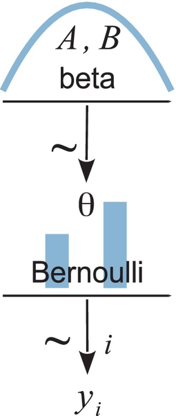
f08-02-9780124058880 — Figure 8.2 Diagram of model with Bernoulli likelihood and beta prior. The pictures of the distributions are intended as stereotypical icons, and are not meant to indicate the exact forms of the distributions. Diagrams like this should be scanned from the bottom up, starting with the data y_i and working upward through the likelihood function and priordistribution. Every arrow in the diagram has a corresponding line of code in a JAGS model specification.

Diagrams like Figure 8.2 should be scanned from the bottom up. This is because models of data always start with the data, then conceive of a likelihood function that describes the data values in terms of meaningful parameters, and finally determine a prior distribution over the parameters. Scanning the diagram from bottom to top may seem awkward at first, but it is necessitated by the conventions for plotting distributions: the dependent value is displayed on the bottom axis and the parameters of the function are best displayed above the bottom axis. If this book's written language were also to flow from bottom to top, instead of from top to bottom, then we would not feel any inconsistency.² To reiterate: when describing a model, the description logically flows from data to likelihood (with its parameters) to prior. If the representational medium is graphs of distributions, then the logical flow goes from bottom to top. If the representational medium is text such as English or computer code, then the logical flow goes from top to bottom.

Diagrams like the one in Figure 8.2 are very useful for two important reasons:

1. They help with conceptual clarity, especially as we deal with more complex models. The diagrams capture the conceptual dependencies among data and parameters without getting bogged down with details of the mathematical formulas for the distributions. Although Equations 8.1 and 8.2 fully specify relations of the variables in the model, the diagram explicitly spatially connects the corresponding variables so that it is easy to visually comprehend the chain of dependencies among variables. Whenever I am creating a model, I draw its diagram to be sure that I really have all its details thought out coherently.

2. The diagrams are very useful for implementing the model in JAGS, because every arrow in the diagram has a corresponding line of code in the JAGS model specification. We will soon see an example of specifying a model in JAGS.

We will now go through a complete example of the sequence of commands in $R$ $R$ that generate an MCMC sample from JAGS for this model. The script that contains the commands is named Jags-ExampleScript.R, in the bundle of programs that accompany this book. You are encouraged to open that script in $R$ $R$ Studio and run the corresponding commands as you read the following sections.

8.2.1 Load data

Logically, models of data start with the data. We must know their basic scale and structure to conceive of a descriptive model. Thus, the first part of a program for analyzing data is loading the data into $R$ $R$ .

In real research, data are stored in a computer data file created by the research. A generic format is text with comma separated values (CSV) on each row. Files of this format usually have a file name with a .csv extension. They can be read into $R$ $R$ with the read.csv function which was introduced in Section 3.5.1 (p. 53). The usual format for data files is one y value per row, with other fields in each row indicating identifying information for the y value, or covariates and predictors of the y value. In the present application, the data values are 1's and 0's from flips of a single coin. Therefore, each row of the data file has a single 1 or 0, with no other fields on each row because there is only one coin.

To bundle the data for JAGS, we put it into a list structure, which was introduced in Section 3.4.4 (p. 51). JAGS will also have to know how many data values there are altogether, so we also compute that total and put it into the list,³ as follows:

myData = read.csv(“z15N50.csv”) # Read the data file; result is a data.frame.
y = myData$y # The y values are the component named y.
Ntotal = length(y) # Compute the total number of flips.
dataList = list( # Put the information into a list.
 y = y.
 Ntotal = Ntotal
)

The syntax in the list may seem strange, because it seems to make tautological statements: y = y and Ntotal = Ntotal. But the two sides of the equal sign are referring to different things. On the left side of the equal sign is the name of that component of the list. On the right side of the equal sign is the value of that component of the list. Thus, the component of the list that says y = y means that this component is named y (i.e., the left side of equal sign) and its value is the value of the variable y that currently exists in $R$ $R$ , which is a vector of 0's and 1's. The component of the list that says Ntotal = Ntotal means that this component is named Ntotal (i.e., the left side of equal sign) and its value is the value of the variable Ntotal that currently exists in $R$ $R$ , which is an integer.

The dataList thereby created in $R$ $R$ will subsequently be sent to JAGS. The list tells JAGS the names and values of variables that define the data. Importantly, the names of the components must match variable names in the JAGS model specification, which is explained in the next section.

8.2.2 Specify model

The diagram in Figure 8.2 is very useful for implementing the model in JAGS, because every arrow in the diagram has a corresponding line of code in the JAGS model specification. The model specification begins with the key word model, and whatever follows, inside curly braces, is a textual description of the dependencies between the variables. Here is the diagram of Figure 8.2 expressed in JAGS:

model {
 for(i in 1:Ntotal ) {
 y[i] ~ dbern( theta ) # likelihood
}
theta ~ dbeta(1, 1) # prior
}

The arrow at the bottom of Figure 8.2, pointing to y_i, is expressed in JAGS as y[i] ~ dbern(theta). Because that relation is true for all instances of y_i, the statement is put inside a for loop. The for loop is merely a shortcut for telling JAGS to copy the statement for every value of i from 1 to Ntotal. Notice that the data-specifying variable names, y and Ntotal, match the names used in the dataList defined in the previous section. This correspondence of names is crucial for JAGS to know the values of the data in the model specification.

The next line in the model statement progresses logically to the specification of the prior, that is, the next arrow up the diagram in Figure 8.2. This particular version uses shape constants of A = 1 and B = 1 in the prior, thus: theta ~ dbeta(1,1).

The model statement progresses logically from likelihood to prior only for the benefit of the human reader. JAGS itself does not care about the ordering of the statements, because JAGS does not execute the model statement as an ordered procedure. Instead, JAGS merely reads in the declarations of the dependencies and then compiles them together to see if they form a coherent structure. The model specification is really just a way of saying, “the ankle bone's connected to the shin bone” and “the shin bone's connected to the knee bone.”⁴ Both statements are true regardless of which one you say first. Thus, the following model specification, which declares the prior first, is equivalent to the model specification above:

model {
theta ~ dbeta(1,1) # prior
for(i in 1:Ntotal ) {
 y[i] ~ dbern( theta ) # likelihood
}
}

While stating the prior first is not a logical problem for JAGS, stating the prior first can be a conceptual problem for humans, for whom it may be difficult to understand the role of theta before knowing it is a parameter in a Bernoulli function, and before knowing that the Bernoulli function is being used to describe dichotomous data.

To get the model specification into JAGS, we create the specification as a character string in $R$ $R$ , then save the string to a temporary text file, and subsequently send the text file to JAGS. Here is the $R$ $R$ code for setting the model specification as a string and writing it to a file arbitrarily named TEMPmodel.txt:

modelString=“# open quote for modelString
model {
for(i in 1:Ntotal ) {
 y[i] ~ dbern( theta )
}
 theta ~ dbeta(1, 1)
}
“ # close quote for modelString
writeLines( modelString, con=“TEMPmodel.txt” ) # write to file

The bundling of the model specification into a string, and saving it to a file, is the same for every model we will ever write for JAGS. Only the model specification changes across applications.

You may have noticed that there was a comment inside modelString, above. JAGS employs comment syntax just like $R$ $R$ . Therefore, we can embed comments in JAGS model specifications, which can be very useful in complicated models. It is worth repeating that the model specification is not interpreted by $R$ $R$ , it is merely a character string in $R$ $R$ . The string is sent to JAGS, and JAGS processes and interprets the model specification.

8.2.3 Initialize chains

This section is about how to specify the starting values of the MCMC chains. JAGS can do this automatically using its own defaults. Therefore, you do not have to fully comprehend this section on a first reading, but you should definitely be aware of it for subsequent review. Although JAGS can automatically start the MCMC chains at default values, the efficiency of the MCMC process can sometimes be improved if we intelligently provide reasonable starting values to JAGS. To do this, we have to figure out values for the parameters in the model that are a reasonable description of the data, and might be in the midst of the posterior distribution.

In general, a useful choice for initial values of the parameters is their maximum likelihood estimate (MLE). The MLE is the value of the parameter that maximizes the likelihood function, which is to say, the value of the parameter that maximizes the probability of the data. The MLE is a reasonable choice because the posterior distribution is usually not radically far from the likelihood function if the prior is noncommittal. For example, review Figure 7.5, p. 167, which showed a case in which the peak of the likelihood function (i.e., the MLE) was not far from the peak of the posterior distribution.

It turns out that for the Bernoulli likelihood function, the MLE is θ = z/N. In other words, the value of θ that maximizes $θ^{z} ? {(1 - θ)}^{(N - z)}$ $θ^{z} ? {(1 - θ)}^{(N - z)}$ is θ = z/N. An example of this fact can be seen in the likelihood function plotted in Figure 6.3, p. 134. For our current application, the data are 0's and 1's in the vector y, and therefore z is sum(y) and N is length(y). We will name the ratio thetaInit, and then bundle the initial value of the parameter in a list that will subsequently get sent to JAGS:

thetaInit = sum(y)/length(y)
initsList = list( theta = thetaInit )

In initsList, each component must be named as a parameter in the JAGS model specification. Thus, in the list statement above, the component name, theta, refers to theta in the JAGS model specification. The initsList is subsequently sent to JAGS.

When there are multiple chains, we can specify different or identical initial values for each chain. The rjags package provides three ways of initializing chains. One way is to specify a single initial point for the parameters, as a single named list as in the example above, and having all chains start there. A second way is to specify a list of lists, with as many sub-lists as chains, and specifying specific initial values in each sub-list. A third way is to define a function that returns initial values when called. (Defining of functions in $R$ $R$ was described in Section 3.7.3, p. 64.) The rjags package calls the function as many times as there are chains. An example of this third method is provided below.

Starting the chains together at the MLE is not universally recommended. Some practitioners recommend starting different chains at greatly dispersed points in parameter space, so that the chains' eventual convergence may be taken as a sign that burn-in has been properly achieved and that the full parameter space has been explored. In particular, this procedure is recommended for interpreting the Gelman- $R$ $R$ ubin convergence statistic. In my experience, however, for the relatively simple models used in this book, appropriate burn-in and convergence is rarely a problem. And, for some complex models, if the chains are initialized at randomly dispersed arbitrary points, they might never converge during a reasonable finite run, with some chains being orphaned indefinitely (although orphaned chains are usually less of a problem in Stan thanin JAGS).

A compromise approach is to start the chains at random points near the MLE. One way to do this is, for each chain, to resample from the data and compute the MLE for the resampled data. $R$ $R$ esampled data will tend to have approximately the same proportion of heads, but sometimes more and sometimes less. Here is an example of a function that returns a named list with a different value for theta every time it is called:

initsList = function() {
 resampledY = sample( y, replace=TRUE )  # resample values from y
 thetaInit = sum(resampledY)/length(resampledY)  # compute proportion (MLE)
 thetaInit = 0.001+0.998*thetaInit  # keep away from 0,1
 return( list( theta=thetaInit ) )  # return as a named list
}

The third line in the function, above, is a protective measure that keeps the initial value of theta in a valid range for JAGS. For example, a prior of beta(θ|2, 2) has zero density at θ = 0 and θ = 1, and JAGS balks at zero prior probabilities, and therefore the chain cannot be started at those extremes.

To demonstrate how the initsList function works, suppose the data y consist of 75% 1's:

> y = c(rep(0,25),rep(1,75))

When the initsList function is called, it returns a list with a component named theta that has a value near75%, as you can see in the following sequence of repeated calls:

> initsList()
$theta
[1] 0.70958
> initsList()
$theta
[1] 0.77944
> initsList()
$theta
[1] 0.72954

8.2.4 Generate chains

Now that we have assembled the data, composed the model specification, and established the initial values of the chains, we are ready to have JAGS actually generate the MCMC sample from the posterior distribution. We do this in three steps. The first step gets all the information into JAGS and lets JAGS figure out appropriate samplers for the model. The next step runs the chains for a burn-in period. Finally, the third step runs and records the MCMC sample that we will subsequently examine.

The first step is accomplished using the jags.model function from the rjags package. This function sends the model specification, data list, and initial-value list to JAGS and tells JAGS to figure out appropriate MCMC samplers. Here is an example of the command:

jagsModel = jags.model( file=“TEMPmodel.txt”, data=dataList, inits=initsList, n.chains=3, n.adapt=500 )

The first argument is the name of the file in which the model specification is stored, that was created at the end of Section 8.2.2. The data argument specifies the list of data that was created in Section 8.2.1. The inits argument specifies the list of initial values that was created in Section 8.2.3. If you want JAGS to create its own initial values for the chains, simply omit the inits argument entirely. The next two arguments specify the number of chains and the number of steps to take for adapting (or tuning) the samplers. These arguments default to 1 chain and 1000 adaptation steps if they are not specified by the user. The jags.model function returns an object that here has been named jagsModel. The object is a list of functions that encapsulate, in JAGS terms, the model and samplers. We will not delve into the jagsModel object. Instead, we merely pass it along to subsequent functions that generate the MCMC sample.

When executing the jags.model command, JAGS checks the model specification, data list, and initial values, for coherence and consistency. If anything is awry, JAGS will issue an error statement. Sometimes the error statements can be cryptic, but they usually contain enough information that you can track down the problem. Sometimes the problem is as simple as a misplaced parenthesis or brace. Sometimes a variable name will be misspelled. Or sometimes you might have a logical problem in the model, or impossible initial values.

After JAGS has created its model, we tell it to run the chains some number of steps to accomplish burn in. We do this by using the update command from package rjags:

update( jagsModel, n.iter=500 )

The first argument is the JAGS object previously created by jags.model. The argument n.iter is the number of iterations, or steps, to take in the MCMC chains. For the present simple application, only a short burn-in is specified. The update function returns no values, it merely changes the internal state of the jagsModel object. It does not record the sampled parameter values during the updating.

After burn-in, we tell JAGS to generate MCMC samples that we will actually use to represent the posterior distribution. The chains of the parameter values are arranged in a specialized format so that various functions from the coda package can be used to examine the chains. Therefore, the function that generates the MCMC samples is called coda.samples in the rjags package. Here is an example of its use:

codaSamples = coda.samples( jagsModel, variable.names=c(“theta”),n.iter=3334 )

As in the update function, the first argument is the JAGS object previously created by jags.model. The argument n.iter is the number of iterations, or steps, taken by each chain. Here, n.iter is set to 3334, which will yield a total of 10,002 steps because there were three chains specified in the jags.model function. Crucially, the variable.names argument specifies which parameters will have their values recorded during the MCMC walk. JAGS will only record the trajectories of parameters that you explicitly tell it to! The variable.names argument must be a vector of character strings. In the present application, there is only one parameter, so the vector has only one element.

The result of the coda.samples function is a coda-formatted object, here named codaSamples, that contains all the sampled parameter values in all the chains. It is a list of matrices. Each component of the list corresponds to a chain, hence in the current example, which has three chains, the list has three components. In each component is a matrix, which has rows indexed by the step in the chain and has columns corresponding to each parameter.

8.2.5 Examine chains

When examining the MCMC samples, the first task is to check that the chains appear to be well mixed and suitably representative of the posterior distribution. Figure 8.3 shows diagnostic information for the θ parameter in our ongoing example. The trace plot in the upper-left panel shows no signs of orphaned chains. The density plot in the lower-right shows that the three subchains are well super-imposed, which is echoed by the Gelman- $R$ $R$ ubin statistic in the lower-left panel being very close to 1.0. The autocorrelation plot in the upper-right panel shows essentially zero autocorrelation for this simple model, and the effective sample size is essentially as large as the full length of the chain.

f08-03-9780124058880 — Figure 8.3 Convergence diagnostics for output of JAGS.

Figure 8.3 was made by a function I created, which, in turn, calls some functions from the coda package. The function I created is named diagMCMC,which stands for diagnostics of MCMC. It is defined in the script called DBDA2E-utilities.R.To use the function, its definition must first be loaded into $R$ $R$ 's working memory:

source(“DBDA2E-utilities.R”)

The source command will only work if the file, DBDA2E-utilities.R, is in $R$ $R$ 's current working directory. Otherwise, you must specify the directory path to the folder in which the file resides, such as, source(“C:/[yourpath]/DBDA2E- utilities.R”). Then the diagnostic-plotting function itself is called:

diagMCMC( codaObject=codaSamples, parName=“theta” )

The diagMCMC function has two arguments. The first specifies the MCMC coda object that was created by JAGS. The second argument specifies which parameter to examine.In models with many parameters, the function is called repeatedly, once for each parameter of interest.

8.2.5.1 The plotPost function

Figure 8.4 shows the MCMC sample from the posterior distribution. It is much like the density plot of Figure 8.3, but plotted as a histogram instead of as a smoothed-density curve, and it is annotated with some different information. Figure 8.4 was created by a function I created called plotPost, which is defined in DBDA2E-utilities.R. The left panel of Figure 8.4 was created using this command:

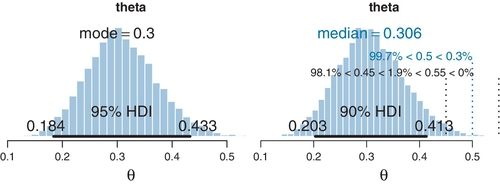
f08-04-9780124058880 — Figure 8.4 Posterior distribution based on output from JAGS, plotted twice using different options in the plotPost function.

plotPost( codaSamples[,”theta”], main=“theta”, xlab=bquote(theta) )

The first argument specified what values to plot; in this case the column named theta from the codaSamples. The plotPost function can take either coda objects or regular vectors for the values to plot. The next arguments merely specify the main title for the plot and the x-axis label. You can see from the plot in the left panel of Figure 8.4 that the annotations default to displaying the estimated mode of the distribution and the estimated 95% HDI. The mode indicates the value of the parameter that is most credible, given the data, but unfortunately the estimate of the mode from an MCMC sample can be rather unstable because the estimation is based on a smoothing algorithm that can be sensitive to random bumps and ripples in the MCMC sample.

The right panel of Figure 8.4 was created using this command:

plotPost( codaSamples[,”theta”], main=“theta”, xlab=bquote(theta),cenTend=“median”, compVal=0.5, ROPE=c(0.45,0.55), credMass=0.90 )

Notice that there were four additional arguments specified. The cenTend argument specifies which measure of central tendency will be displayed; the options are “mode”,“median”, and “mean”. The mode is most meaningful but also unstable in its MCMC approximation. The median is typically the most stable. The compVal argument specifies a “comparison value.” For example, we might want to know whether the estimated bias differs from the “fair” value of θ = 0.5. The plot shows the comparison value and annotates it with the percentage of the MCMC sample below or above the comparison value. The next argument specifies the limits of the region of practical equivalence, which will be discussed in depth in Section 12.1.1. For now, we merely note that it is a buffer interval around the comparison value, and the plot annotates its limits with the percentage of the distribution below, within, and above the region of practical equivalence. Finally, the credMass argument specifies the mass of the HDI to display. It defaults to 0.95, but here I have specified 0.90 instead merely to illustrate its use.

The plotPost function has other optional arguments. The argument HDItextPlace specifies where the numerical labels for the HDI limits will be placed. If HDItextPlace=0, the numerical labels are placed completely inside the HDI. If HDItextPlace=1, the numerical labels are placed completely outside the HDI. The default is HDItextPlace=0.7, so that the labels fall 70% outside the HDI. The argument showCurve is a logical value which defaults to FALSE. If showCurve=TRUE, then a smoothed kernel density curve is displayed instead of a histogram.

The plotPost function also takes optional graphical parameters that get passed to $R$ $R$ 's plotting commands. For example, when plotting histograms, plotPost defaults to putting white borders on each bar. If the bars happen to be very thin, the white borders can obscure the thin bars. Therefore, the borders can be plotted in a color that matches the bars by specifying border=“skyblue”. As another example, sometimes the default limits of the x-axis can be too extreme because the MCMC chain happens to have a few outlying values. You can specify the limits of the x-axis using the xlim argument, such as xlim=c(0,1).

8.3 Simplified scripts for frequently used analyses

As was mentioned at the beginning of this example, several pages back, the complete script for the preceding analysis is available in the file Jags-ExampleScript.R. It is valuable for you to understand all the steps involved in the script so you know how to interpret the output and so you can create scripts for your own specialized applications in the future. But dealing with all the details can be unwieldy and unnecessary for typical, frequently used analyses. Therefore, I have created a catalog of simplified, high-level scripts.

The scripts in the catalog have elaborate names, but the naming structure allows an extensive array of applications to be addressed systematically. The file naming system works as follows. First, all scripts that call JAGS begin with “Jags -.” Then the nature of the modeled data is indicated. The modeled data are generically called y in mathematical expressions, so the file names use the letter “Y” to indicate this variable. In the present application, the data are dichotomous (i.e., 0 and 1), and therefore the file name begins with “Jags-Ydich-.” The next part of the file name indicates the nature of the predictor variables, sometimes also called covariates or regressors, and generically called x in mathematical expressions. In our present application, there is only a single subject. Because the subject identifier is a nominal (not metric) variable, the file name begins with “Jags-Ydich-Xnom1subj-.” Finally, the nature of the model is indicated. In the present application, we are using a Bernoulli likelihood with beta prior, so we complete the file name as “Jags-Ydich-Xnom1subj-MbernBeta.R.” Other scripts in the catalog use different descriptors after Y, X, and M in their file names. The file Jags-Ydich-Xnom1subj-MbernBeta.R defines the functions that will be used, and the file Jags-Ydich-Xnom1subj-MbernBeta-Example.R contains the script that calls the functions.

What follows below are condensed highlights from the script Jags-Ydich-Xnom1subj-MbernBeta-Example.R. Please read through it, paying attention to the comments.

# Load the data
myData = read.csv(“zl5N50.csv”) # must have a component named y
# Load the functions genMCMC, smryMCMC, and plotMCMC:
source(“Jags-Ydich-Xnom1subj-MbernBeta.R”)
# Generate the MCMC chain:
mcmcCoda = genMCMC( data=myData, numSavedSteps=l0000 )
# Display diagnostics of chain, for specified parameter:
diagMCMC( mcmcCoda, parName=“theta” )
# Display numerical summary statistics of chain:
smryMCMC( mcmcCoda )
# Display graphical posterior information:
plotMCMC( mcmcCoda, data=y )

Notice that the JAGS process–that was previously an extensive script that assembled the data list, the model specification, the initial values, and the running of the chains– has here been collapsed into a single function called genMCMC. Hooray! Thus, by using this script, you can analyze any data that have this structure merely by reading in the appropriate data file at the beginning, and without changing anything else in the script.

The high-level scripts should operate without changes for any data file structured in the way expected by the function genMCMC. If you want to change the functions in some way, then you will probably need to do some debugging in the process. Please review the section on debugging functions, back in Section 3.7.6 (p. 67).

8.4 Example: difference of biases

In the previous chapter, we also estimated the difference of biases between coins (or subjects). It is easy to implement that situation in JAGS. This section will first illustrate the model structure and its expression in JAGS, and then show the high-level script that makes it easy to run the analysis for any data structured this way.

As usual, we start our analysis with the structure of the data. In this situation, each subject (or coin) has several trials (or flips) that have dichotomous (0/1) outcomes. The data file therefore has one row per measurement instance, with a column for the outcome y and a column for the subject identifier s. For example, the data file might look like this:

y.s
1,Reginald
0,Reginald
1,Reginald
1,Reginald
1,Reginald
1,Reginald
1,Reginald
0,Reginald
0,Tony
0,Tony
1,Tony
0,Tony
0,Tony
1,Tony
0,Tony

Notice that the first row contains the column names (y and s), and the columns are comma-separated. The values under y are all 0's or 1's. The values under s are unique identifiers for the subjects. The column names must come first, but after that, the rows can be in any order.

The program reads the CSV file and converts the subject identifiers to consecutive integers so that they can be used as indices inside JAGS:

myData = read.csv(“z6N8z2N7.csv”)
y = myData$y
s = as.numeric(myDataSs) # converts character to consecutive integer levels

The result of the above is a vector y of 0's and 1's, and a vector s of 1's for $R$ $R$ eginald followed by 2's for Tony. (The conversion of factor levels to integers was discussed in Section 3.4.2, following p. 46.) Next, the data are bundled into a list for subsequent shipment to JAGS:

Ntotal = length(y)
Nsubj = length(unique(s))
dataList = list(
 y = y,
 s = s,
 Ntotal = Ntotal,
 Nsubj = Nsubj
)

To construct a model specification for JAGS, we first make a diagram of the relations between variables. The data consist of observed outcomes y_i|s, where the subscript refers to instances i within subjects s. For each subject, we want to estimate their bias, that is, their underlying probability of generating an outcome 1, which we will denote θ_s. We model the data as coming from a Bernoulli distribution:

$y_{i} | s \sim dbern (θ_{s})$ $y_{i} | s \sim dbern (θ_{s})$

and this corresponds with the lower arrow in Figure 8.5. Each subject's bias, θ_s, has an independent beta-distributed prior:

$θ_{s} \sim dbeta (A, B)$ $θ_{s} \sim dbeta (A, B)$

and this corresponds with the upper arrow in Figure 8.5. To keep the example consistent with the earlier demonstrations, we set A = 2 and B = 2 (recall the use of a beta(θ|2, 2) prior in Figure 7.5, p. 167, Figure 7.6, p. 169, and Figure 7.8, p. 174).

f08-05-9780124058880 — Figure 8.5 Diagram of model with Bernoulli likelihood and beta prior for multiple subjects, s. Notice the indices on the variables and arrows. Every arrow in the diagram has a corresponding line of code in JAGS model specification.

Having created a diagram for the model, we can then express it in JAGS:

model {
 for(i in l: Ntotal ) {
 y[i] ~ dbern( theta[s[i]] ) # notice nested indexing
 }
 for(s in l: Nsubj ) {
 theta[s] ~ dbeta(2,2)
 }
}

In the above code, notice that the index i goes through the total number of data values, which is the total number of rows in the data file. So you can also think of i as the row number. The important novelty of this model specification is the use of “nested indexing” for theta[s[i]] in the dbern distribution. For example, consider when the for loop gets to i = 12. Notice from the data file that s[12] is 2. Therefore, the statement y[i] ~ dbern(theta[s[i]]) becomes y[12] ~ dbern(theta[s[12]]) which becomes y[12] ~ dbern(theta[2]). Thus, the data values for subject s are modeled by the appropriate corresponding θ_s.

The details of the JAGS model specification were presented to show how easy it is to express the model in JAGS. JAGS then does the MCMC sampling on its own! There is no need for us to decide whether to apply a Metropolis sampler or a Gibbs sampler, and no need for us to build a Metropolis proposal distribution or derive conditional distributions for a Gibbs sampler. JAGS figures that out by itself.

The JAGS program for this data structure has been assembled into a set of functions that can be called from a high-level script, so you do not have to mess with the detailed model specification if you do not want to. The high-level script is analogous in structure to the example in the previous section. The only thing that changes is the script file name, which now specifies Ssubj instead of 1subj, and, of course, the data file name. What follows below are condensed highlights from the script Jags-Ydich-XnomSsubj-MbernBeta-Example.R. Please read through it, paying attention to the comments.

# Load the data
myData = read.csv(“z6N8z2N7.csv”) # myData is a data frame.
# Load the functions genMCMC, smryMCMC, and plotMCMC:
source(“Jags-Ydich-XnomSsubj-MbernBeta.R”)
# Generate the MCMC chain:
mcmcCoda = genMCMC( data=myData, numSavedSteps=l0000 )
# Display diagnostics of chain, for specified parameter:
diagMCMC( mcmcCoda, parName=“theta[l]” )
# Display numerical summary statistics of chain:
smryMCMC( mcmcCoda, compVal=NULL, compValDiff=0.0 )
# Display graphical posterior information:
plotMCMC( mcmcCoda, data=myData, compVal=NULL, compValDiff=0.0 )

The overall structure of the script is the same as the previous high-level script for the single-subject data. In particular, the functions genMCMC, smryMCMC, and plotMCMC have the same names as the previous script, but they are defined differently to be specific to this data structure. Therefore, it is crucial to source the appropriate function definitions (as is done above) before calling the functions.

Figure 8.6 shows the result of the plotMCMC function. It displays the marginal distribution of each individual parameter and the difference of the parameters. It also annotates the distributions with information about the data. Specifically, the value of z_s/N_s is plotted as a large “+” symbol on the horizontal axis of each marginal distribution, and the value z₁/N₁-z₂/N₂ is plotted on the horizontal axis of the difference distribution. The difference distribution also plots a reference line at zero, so we can easily see the relation of zero to the HDI.

f08-06-9780124058880 — Figure 8.6 Posterior distribution created by JAGS. Compare the upper-right panel with Figure 7.9.

If you compare the upper-right panel of Figure 8.6 with the results from Figure 7.9 (p. 177), you can see that JAGS produces the same answer as our “home grown” Metropolis and Gibbs samplers.

8.5 Sampling from the prior distribution in jags

There are various reasons that we may want to examine the prior distribution in JAGS:

• We might want to check that the implemented prior actually matches what we intended:

• For example, perhaps what we imagine a beta(θ| A, B) prior looks like is not really what it looks like.

• Or, perhaps we simply want to check that we did not make any programming errors.

• Or, we might want to check that JAGS is functioning correctly. (JAGS is well developed, and we can have high confidence that it is functioning correctly. Yet, as the proverb says, “trust but verify.”⁵)

• We might want to examine the implied prior on parameter combinations that we did not explicitly specify. For example, in the case of estimating the difference of two biases, we put independent beta(θ |A, B) priors on each bias separately, but we never considered what shape of prior that implies for the difference of biases, θ1 – θ2. We will explore this case below.

• We might want to examine the implied prior on mid-level parameters in hierarchical models, when the explicit prior was specified on higher-level parameters. We will use hierarchical models extensively in later chapters and will see an example of this in Section 9.5.1.

It is straight forward to have JAGS generate an MCMC sample from the prior: We simply run the program with no data included. This directly implements the meaning of the prior, which is the allocation of credibility across parameter values without the data. Intuitively, this merely means that when there are no new data, the posterior is the prior, by definition. Another way to conceptualize it is by thinking of the likelihood function for null data as yielding a constant value. That is, $p (\emptyset | θ) = k$ $p (\emptyset | θ) = k$ a constant (greater than zero). You can think of this as merely an algebraic convenience, or as a genuine probability that the data-sampling process happens to collect no data. In either case, notice that it asserts that the probability of collecting no data does not depend on the value of the parameter. When a constant likelihood is plugged into Bayes' rule (Equation 5.7, p. 106), the likelihood cancels out (in numerator and denominator) and the posterior equals the prior.

To run JAGS without the data included, we must omit the y values, but we must retain all constants that define the structure of the model, such as the number of (absent) data values and the number of (absent) subjects and so forth. Thus, at the point in the program that defines the list of data shipped to JAGS, we comment out only the line that specifies y. For example, in Jags-Ydich-XnomSsubj-MbernBeta.R, comment out the data, y, but retain all the structural constants, like this:

dataList = list(
#y = y,
 s = s,
 Ntotal = Ntotal,
 Nsubj = Nsubj
)

Then just run the program with the usual high-level script. Be sure you have saved the program so that the high-level script calls the modified version. Also be sure that if you save the output you use file names that indicate they reflect the prior, not the posterior.

Figure 8.7 shows the prior sampled by JAGS. Notice that the distributions on the individual biases (θ₁ and θ₂) are, as intended, shaped like beta(θ|2,2) distributions (cf. Figure 6.1, p. 128). Most importantly, notice the implied prior on the difference of biases, shown in the upper-right panel of Figure 8.7. The prior does not extend uniformly across the range from − 1 to +1, and instead shows that extreme differences are suppressed by the prior. This might or might not reflect the intended prior on the difference. Exercise 8.4 explores the implied prior on θ₁ – θ₂ for different choices of priors on θ₁ and θ₂ individually.

f08-07-9780124058880 — Figure 8.7 The prior distribution for difference of biases. Compare with Figure 8.6.

8.6 Probability distributions available in jags

JAGS has a large collection of frequently used probability distributions that are built-in. These distributions include the beta, gamma, normal, Bernoulli, and binomial along with many others. A complete list of distributions, and their JAGS names, can be found in the JAGS user manual.

8.6.1 Defining new likelihood functions

Despite the breadth of offerings, there may be occasions when you would like to use a probability distribution that is not built into JAGS. In particular, how can we get JAGS to use a likelihood function that is not prepackaged? One way is to use the so-called “Bernoulli ones trick” or the analogous “Poisson zeros trick” (e.g., Lunn et al., 2013).

Suppose we have some likelihood function, p(y|parameters), for which we have a mathematical formula. For example, the normal probability distribution has a mathematical formula specified in Equation 4.4, p. 84. Suppose, however, that JAGS has no built-in probability density function (pdf) of that form. Therefore, unfortunately, we cannot specify in JAGS something like y[i] ~ pdf(parameters), where “pdf”stands for the name of the probability density function we would like.

To understand what we will do instead, it is important to realize that what we would get from y[i] ~ pdf(parameters) is the value of the pdf when y[i] has its particular value and when the parameters have their particular randomly generated MCMC values. All we need to do is specify any valid JAGS code that yields that result.

Here is the “Bernoulli ones trick.” First, notice that dbern(1|θ) = θ. In other words, if we write JAGS code 1 ~ dbern( theta ), it yields a likelihood that is the value of theta. If we define, in another line of JAGS code, the value of theta as the desired likelihood at y[i], then the result is the likelihood at y[i] . Thus, the JAGS model statements together yield the same thing as y[i] ~ pdf ( parameters ). The variable name spy[i] stands for scaled probability of y_i.

spy[i] <- pdf( y[i], parameters)/C# where pdf is a formula
l ~ dbern( spy[i] )

Important caveat: the value of the parameter in dbern must be between zero and one, and therefore the value of spy[i] must be scaled so that, no matter what the random parameter values happen to be, spy[i] is always less than 1. We achieve this by dividing by a large positive constant C, which must be determined separately for each specific application. It is okay to use a scaled likelihood instead of the correct-magnitude likelihood because MCMC sampling uses only relative posterior densities of current and proposed positions, not absolute posterior densities.

In JAGS, the vector of 1's must be defined outside the model definition. One way to do that is with a data block that precedes the model block in JAGS:

data {
 C <- 10000 # JAGS does not warn if too small!
 for (i in 1:N) {
 ones[i] <- 1
 }
}
model {
 for (i in 1:N) {
 spy[i] <- pdf( y[i], parameters )/C # where pdf is a formula
 ones[i] ~ dbern( spy[i] )
 }
 parameters ~ dprior...
}

As a specific example, suppose that the values of y are continuous metric values, and we want to describe the data as a normal distribution. Suppose that JAGS had no dnorm built into it. We could use the method above, along with the mathematical formula for the normal density from Equation 4.4 (p. 84). Therefore, we would specify

spy[i] <- (exp(-0.5*((y[i]-mu)/sigmaˆ2)/(sigma*(2*3.1415926ˆ0.5))/C

Alternatively, there is the “Poisson zeros trick” which uses the same approach but with the fact that dpois(0,θ) = exp(–θ). Therefore, the JAGS statement 0 ~ dpois( -log(theta[i]) ) yields the value theta[i]. So we can define theta[i] = pdf(y[i],parameters) and put -log(theta[i]) into dpois to get the desired likelihood value in JAGS. But notice that - log(theta[i]) must be a positive value (to be valid for the Poisson distribution), therefore the likelihood must have a constant added to it to be sure it is positive no matter what values of y[i] and parameters gets put into it.

Finally, with a bit of programming effort, JAGS can be genuinely extended with new distributions, completely bypassing the tricks above. The runjags package implements a few additional probability densities and explains a way to extend JAGS (see Denwood, 2013). Another approach to extending JAGS is explained by Wabersich and Vandekerckhove (2014).

8.7 Faster sampling with parallel processing in runjags

Even when using multiple chains in JAGS, each chain is computed sequentially on a single central processing unit, or “core,” in the computer. At least, that is the usual default procedure for JAGS called from rjags. But most modern computers have multiple cores. Instead of using only one core while the others sit idle, we can run chains in parallel on multiple cores, thereby decreasing the total time needed. For example, suppose we desire 40,000 total steps in the chain. If we run four chains of 10,000 steps simultaneously on four cores, it takes only about 1/4th the time as running them successively on a single core. (It is a bit more than the reciprocal of the number of chains because all the chains must be burned in for the full number of steps needed to reach convergence.) For the simple examples we have explored so far, the time to run the MCMC chains is trivially brief. But for models involving large data sets and many parameters, this can be a huge time savings.

The package runjags (Denwood, 2013) makes it easy to run parallel chains in JAGS. The package provides many modes for running JAGS, and a variety of other facilities, but here I will focus only on its ability to run chains in parallel on multiple processors. For more information about its other abilities, see the article by Denwood (2013) and the runjags manual available at http://cran.r-project.org/web/packages/runjags/.

To install the runjags package into $R$ $R$ , follow the usual procedure for installing packages. At $R$ $R$ 's command line, type

install.packagesC'runjags”)

You only need to do that once. Then, for any session in which you want to use the runjags functions, you must load the functions into $R$ $R$ 's memory by typing

library(“runjags”)

With runjags loaded into $R$ $R$ 's working memory, you can get more information about it by typing ?runjags at the command line.

The essential difference between running JAGS via rjags and runjags is merely the functions used to invoke JAGS. As an example, suppose our script has already defined the model as the file model.txt,the data list as dataList, and the initial values as a list or function initsList. Then, suppose the script specifies the details of the chains as follows:

nChains=3
nAdaptSteps=l000
nBurninSteps=500
nUseSteps=l0000 # total number of used steps
nThinSteps=2

If we were calling JAGS via rjags, we could use this familiar sequence of commands:

library(rjags)
 jagsModel = jags.model(file=“model.txt”,
 data=dataList,
 inits=initsList,
 n.chains=nChains,
 n.adapt=nAdaptSteps )
update(  jagsModel,
 n.iter=nBurninSteps )
codaSamples = coda.samples( jagsModel,
 variable.names=c(“theta”),
 n.iter=ceiling(nUseSteps*nThinSteps/nChains),
 thin=nThinSteps )

Across the sequence of three commands above, I aligned the arguments vertically, with one argument per line, so that you could easily see them all. To call JAGS via runjags, we use the same argument values like this:

library(runjags)
runJagsOut <- run.jags( method=“parallel”,
 model=“model.txt”,
 monitor=c(“theta”),
 data=dataList,
 inits=initsList,
 n.chains=nChains,
 adapt=nAdaptSteps,
 burnin=nBurninSteps,
 sample=ceiling(nUseSteps/nChains),
 thin=nThinSteps,
 summarise=FALSE,
 plots=FALSE )
codaSamples = as.mcmc.list( runJagsOut )

A key advantage of runjags is specified by the first argument in the run.jags command above, named method. This is where we can tell runjags to run parallel chains on multiple cores. The method argument has several options, which you can read about in the help file. For our purposes, the two options of primary interest are “rjags,” which runs in ordinary rjags mode, and “parallel,” which runs the chains in parallel on different computer cores.

Some of the arguments are slightly renamed in runjags relative to rjags, but the correspondence is easy to understand, and there is detailed help available by typing ?run.jags at $R$ $R$ 's command line (and in the runjags manual, of course). For example, the argument for specifying the number of steps to take after burnin is n.iter in rjag's coda.samples command, and corresponds to sample in runjag's run.jags command, but because of the way thinning is implemented, the values must be adjusted as shown. (This is for rjags version 3-12 and runjags version 1.2.0-7; beware of the possibility of changes in subsequent versions.)

Thereare twonew arguments in the run.jags command: summarise and plots. The summarise argument tells runjags whether or not to compute diagnostic statistics for every parameter. The diagnostics can take a long time to compute, especially for models with many parameters and long chains. The summarise argument has a default value of TRUE. Be careful, however, to diagnose convergence in other ways when runjags is told not to.

After run.jags returned its output, the final line of code, above, converted the runjags object to coda format. This conversion allows coda-oriented graphical functions to be used later in the script.

Some important caveats: if your computer has K cores, you will usually want to run only K − 1 chains in parallel, because while JAGS is running you will want to reserve one core for other uses, such as word processing, or answering email, or watching cute puppy videos to improve your productivity (Nittono, Fukushima, Yano, & Moriya, 2012). If you use all K cores for running JAGS, your computer may be completely swamped by those demands and effectively lock you out until it is done.⁶ Another important consideration is that JAGS has only four distinct (pseudo-)random number generators ( $R$ $R$ NGs). If you run up to four parallel chains, runjags (and rjags too) will use four different $R$ $R$ NGs, which gives some assurance that the four chains will be independent. If you run more than four parallel chains, however, you will want to explicitly initialize the $R$ $R$ NGs to be sure that you are generating different chains. The runjags manual suggests how to do this.

“Okay,” you may be saying, “that's all terrific, but how do I know how many cores my computer has?” One way is by using a command in $R$ $R$ from the parallel package, which gets installed along with runjags. At the $R$ $R$ command prompt, type library(“parallel”) to load the package, then type detectCores(), with the empty parentheses.

8.8 Tips for expanding jags models

Often, the process of programming a model is done is stages, starting with a simple model and then incrementally incorporating complexifications. At each step, the model is checked for accuracy and efficiency. This procedure of incremental building is useful for creating a desired complex model from scratch, for expanding a previously created model for a new application, and for expanding a model that has been found to be inadequate in a posterior predictive check. The best way to explain how to expand a JAGS model is by example. Section 17.5.2 (p. 507) summarizes the necessary steps, exemplified by expanding a linear regression model to a quadratic trend model.

8.9 Exercises

Look for more exercises at (https://sites.google.com/site/doingbayesiandataanalysis/

Exercise 8.1

[Purpose: $R$ $R$ un the high level scripts with other data to see how easy they are.] Consider the high-level script, Jags-Ydich-XnomSsubj-MbernBeta-Example. $R$ $R$ . For this exercise, you will use that script with a new data file, and notice that you only need to change a single line, namely the one that loads the data file.

In $R$ $R$ Studio, open a new blank file by selecting the menu items File → New → Text file. Manually type in new fictional data in the same format as the data shown in Section 8.4, p. 208, but with three subjects instead of two. Use whatever names you fancy, and as many trials for each subject as you fancy. Perhaps put a preponderance of 0's for one subject and a preponderance of 1's for another subject. Use a lot of trials of one subject, and relatively few trials for another. Save the file with a filename that ends with “.csv.” Then, in the script, use that file name in the read.csv command. In your report, include the data file and the graphical output of the analysis. Are the estimates reasonable? What is the effect of different sample sizes for the estimates of different subjects?

Exercise 8.2

[Purpose: Pay attention to the output of smryMCMC.] The graphical plots from plotMCMC are useful for understanding, but they lack some numerical details. $R$ $R$ un the high-level script, Jags-Ydich-XnomSsubj-MbernBeta-Example. $R$ $R$ , and explain the details in the output from smryMCMC. Explain what the rope and ropeDiff arguments do.

Exercise 8.3

[Purpose: Notice what gets saved by the high-level scripts.] $R$ $R$ un the high-level script, Jags-Ydich-XnomSsubj-MbernBeta-Example. $R$ $R$ , and notice what files are created (i.e., saved) in your compute $R$ $R$ 's working directory. Explain what these files are, and why they might be useful for future reference. Hint: In the file Jags-Ydich-XnomSsubj-MbernBeta. $R$ $R$ , search for the word “save.”