17.2.1 Robust linear regression in JAGS

As has been emphasized (e.g., at the end of Section 8.2), hierarchical dependency diagrams like Figure 17.2 are useful not only for conceptualizing the structure of a model but also for programming it. Every arrow in Figure 17.2 has a corresponding line of code in JAGS or Stan. The following sections describe implementations of the model. The core of the model specification for JAGS is virtually an arrow-to-line transliteration of the diagram. The seven arrows in Figure 17.2 have seven corresponding lines of code:

model {
 for ( i in 1:Ntotal ) {
 zy[i] ∼ dt( mu[i] , 1/zsigmaˆ2 , nu )
 mu[i] <- zbeta0 + zbeta1 * zx[i]
 }
 zbeta0 ∼ dnorm( 0 , 1/(10)ˆ2 )
 zbeta1 ∼ dnorm( 0 , 1/(10)ˆ2 )
 zsigma ∼ dunif( 1.0E-3 , 1.0E+3 )
 nu <- nuMinusOne+1
 nuMinusOne ∼ dexp(1/29.0)
}

Some of the parameter names in the code above are preceded by the letter “z” because the data will be standardized before being sent to the model, as will be described later, and standardized data often are referred to by the letter “z.”

One of the nice features of JAGS (and Stan) is that arguments in distributions are functionally evaluated, so we can put a statement with operations in the place of an argument instead of only a variable name. For example, in the dt distribution earlier, the precision argument has the expression 1/zsigmaˆ2 instead of just a variable name. We could do the same thing for dt's other arguments. In particular, instead of assigning a value to mu[i] on a separate line, we could simply insert zbeta0 + zbeta1 * zx[i] in place of mu[i] in the mean argument of dt. Thus, assignment arrows in diagrams like Figure 17.2 do not necessarily need a separate line in the JAGS code. However, when the expression is put directly into an argument, JAGS cannot record the value of the expression throughout the chain. Thus, in the form shown earlier, mu[i] is available for recording along with the parameter values at every step. We are not interested in mu[i] at every step; therefore, the revised code (exhibited later) will put its expression directly into the mean argument of dt. On the other hand, the expression for nu will remain on a separate line (as shown above) because we do want an explicit record of its value.

data {
 Ntotal <- length(y)
 xm <- mean(x)
 ym <- mean(y)
 xsd <- sd(x)
 ysd <- sd(y)
 for ( i in 1:length(y) ) {
 zx[i] <- ( x[i] - xm ) / xsd
 zy[i] <- ( y[i] - ym ) / ysd
 }
}

model {
 for ( i in 1:Ntotal ) {
 zy[i] ∼ dt( zbeta0 + zbeta1 * zx[i] , 1/zsigmaˆ2 , nu )
 }
 # Priors vague on standardized scale:
 zbeta0 ∼ dnorm( 0 , 1/10ˆ2 )
 zbeta1 ∼ dnorm( 0 , 1/10ˆ2 )
 zsigma ∼ dunif( 1.0E-3 , 1.0E+3 )
 nu <- nuMinusOne+1
 nuMinusOne ∼ dexp(1/29.0)
 # Transform to original scale:
 beta1 <- zbeta1 * ysd / xsd
 beta0 <- zbeta0 * ysd + ym - zbeta1 * xm * ysd / xsd
 sigma <- zsigma * ysd
}

17.2.2 Robust linear regression in Stan

$\text{R}$ecall from Section 14.1 (p. 400) that Stan uses Hamiltonian dynamics to find proposed positions in parameter space. The trajectories use the gradient of the posterior distribution to move large distances even in narrow distributions. Thus, HMC by itself, without data standardization, should be able to efficiently generate a representative sample from the posterior distribution.

data {
 int<lower=1> Ntotal ;
 real x[Ntotal] ;
 real y[Ntotal] ;
 real meanY ;
 real sdY ;
 real meanX ;
 real sdX ;
}
transformed data { // for constants in priors
 real unifLo ;
 real unifHi ;
 real expLambda ;
 real beta0sigma ;
 real beta1sigma ;
 unifLo <- sdY/1000 ;
 unifHi <- sdY*1000 ;
 expLambda <- 1/29.0 ;
 beta1sigma <- 10*fabs(sdY/sdX) ; // fabs is absolute value
 beta0sigma <- l0*fabs(meanX*sdY/sdX) ;
}
parameters {
 real beta0 ;
 real beta1 ;
 real<lower=0> nuMinusOne ;
 real<lower=0> sigma ;
}
transformed parameters {
 real<lower=0> nu ; // actually lower=1
 nu <- nuMinusOne + 1 ;
}
model {
 sigma ∼ uniform( unifLo , unifHi ) ;
 nuMinusOne ∼ exponential( expLambda ) ;
 beta0 ∼ normal( 0 , beta0sigma ) ;
 beta1 ∼ normal( 0 , beta1sigma ) ;
 for ( i in 1:Ntotal ) {
 y[i] ∼ student_t( nu , beta0 + beta1 * x[i] , sigma ) ;
 }
}

17.2.3 Stan or JAGS?

The Stan and JAGS implementations were both run on the data in Figure 17.4, and they produced very similar results in terms of the details of the posterior distribution. For a comparison, both implementations were run with 500 adaptation steps, 1000 burn-in steps, and 20,000 saved steps with no thinning, using four chains. On my modest desktop computer, a run in JAGS took about 180 seconds, while a run in Stan (including compilation) took about 485 seconds (2.7 times as long). The ESS in JAGS was quite different for different parameters, being about 5000 for v and σ but about 16,000 for β₀ and β₁. The effective sample size (ESS) in Stan was more consistent across parameters but not as high as JAGS for some, being about 8000 for v and σ but only about 7000 for β₀ and β₁.

Thus, Stan does indeed go a long way toward solving the correlated-parameter problem for which JAGS needed the intervention of standardizing the data. Stan also samples the normality and scale parameters with less autocorrelation than JAGS, as we saw previously in Figure 16.10 (p. 467). HMC deftly navigates through posterior distributions where other samplers may have troubles. But Stan took longer in real time and yielded a smaller ESS for the main parameters of interest, namely the slope and intercept. Stan's efficiency with this model might be improved if we used standardized data as we did for JAGS, but a main point of this demonstration was to show that HMC is able to navigate difficult posterior distributions. Stan's efficiency (and JAGS') might also be improved if the t distribution were reparameterized, as explained in the Stan Reference Manual. Although subsequent programs in this section focus on JAGS, keep in mind that it is straight forward to translate the programs into Stan.

17.2.4 Interpreting the posterior distribution

Now that we are through all the implementation details, we will discuss the results of the analysis shown in Figures 17.3 and 17.4. Recall that both figures show results from the same data generator, but Figure 17.3 has only 30 data points while Figure 17.4 has 300. By comparing the marginal distributions of the posterior across the two figures, you can see that the modal estimates of the slope, intercept, and scale are about the same, but the certainty of the estimate is much tighter for 300 data points than for 30 data points. For example, with N = 30, the slope has modal estimate of about 4.5 (pounds per inch), with a 95% HDI that extends from about 2.0 to 7.0. When N = 300, again the slope has modal estimate of about 4.5, but the 95% HDI is narrower, extending from about 3.6 to 5.2.

It is interesting to note that the normality parameter does not have the same estimate for the two data sets. As the data set gets bigger, the estimate of the normality parameter gradually gets smaller, overcoming the prior which remains fairly dominant with N = 30. ($\text{R}$ecall the discussion of the exponential prior on v in Section 16.2.1, p. 462.) With larger data sets, there is more opportunity for outliers to appear, which are inconsistent with large values of v. (Of course, if the data are genuinely normally distributed, then larger data sets just reinforce large values of the normality parameter.)

In some applications, there is interest in extrapolating or interpolating trends at x values sparsely represented in the current data. For instance, we might want to predict the weight of a person who is 50 inches tall. A feature of Bayesian analysis is that we get an entire distribution of credible predicted values, not only a point estimate. To get the distribution of predicted values, we step through the MCMC chain, and at each step, we randomly generate simulated data from the model using the parameter values at that step. You can think of this by looking at the vertically plotted noise distributions in Figure 17.4. For any given value of height, the noise distributions show the credible predicted values of weight. By simulating data from all the steps in the chain, we integrate over all those credible noise distributions. An interesting aspect of the predictive distributions is that they are naturally wider, that is, less certain, the farther away we probe from the actual data. This can be seen most easily in Figure 17.3. As we probe farther from the data, the spread between credible regression lines gets larger, and thus the predicted value gets less certain.

The upper panels of Figures 17.3 and 17.4 show the data with a smattering of credible regression lines and t distributions superimposed. This provides a visual posterior predictive check, so we can qualitatively sense whether there are systematic deviations of the data from the form implied by the model. For example, we might look for nonlinear trends in the data or asymmetry in the distribution of weights. The data suggest that there might be some positive skew in the distribution of weights relative to the regression lines. If this possibility had great theoretical importance or were strong enough to cast doubt on the interpretation of the parameters, then we would want to formulate a model that incorporated skew in the noise distribution. For more information about posterior predictive checks, see Kruschke (2013b). Curiously, in the present application, the robust linear-regression model does a pretty good job of mimicking the data, even though the data were actually generated by three bivariate normal distributions. $\text{R}$emember, though, that the model only mimics the dependency of y on x, and the model does not describe the distribution of x.

17.3.1 The model and implementation in JAGS

Figure 17.6 shows a diagram of the model. It might seem a bit daunting, but if you compare it with Figure 17.2 on p. 480 you will see that it merely adds a level to the basic model we are already very familiar with. The diagram is useful for understanding all the dependencies in the model, and for programming in JAGS (and Stan) because every arrow in the diagram has a corresponding line in the JAGS model specification.

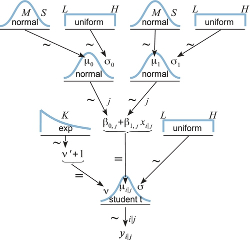
Starting at the bottom of Figure 17.6, we see that the ith datum within the jth subject comes from a t distribution that has a mean of μ_i|j = β_0,j+ β_1,jx_i|j. Notice that the intercept and slope are subscripted with j, meaning that every subject has its own slope and intercept. Moving up the hierarchical diagram, we see that the slopes across the individuals all come from a higher-level normal distribution that has mean denoted μ₁ and standard deviation of σ₁, both of which are estimated. In other words, the model assumes that β_1,j∼ normal(μ₁, σ₁), where μ₁ describes the typical slope of the individuals and σ₁ describes the variability of those individual slopes. If every individual seems to have nearly the same slope, then σ₁ is estimated to be small, but if different individuals have very different slopes, then σ₁ is estimated to be large. Analogous considerations apply to the intercepts. At the top level of the hierarchy, the group-level parameters are given generic vague priors.

This model assumes that the standard deviation of the noise within each subject is the same for all subjects. In other words, there is a single σ parameter, as shown at the bottom of Figure 17.6. This assumption could be relaxed by providing subjects with distinct noise parameters, all under a higher level distribution. We will see our first example of this approach later, in Figure 19.6 (p. 574).

To understand the JAGS implementation of the model, we must understand the format of the data file. The data format consists of three columns. Each row corresponds to one point of data and specifies the x, y values of the point and the subject who contributed that point. For the ith row of the data file, the x value is x[i], the y value is y[i], and the subject index j is s[i]. Notice that the index i in the JAGS model specification is the row of overall data file, not the ith value within subject j. The model specification assumes that the subject indices are consecutive integers, but the data file can use any sort of unique subject identifiers because the identifiers get converted to consecutive integers inside the program. The subject indices will be used to keep track of individual slopes and intercepts.

The JAGS implementation of this model begins by standardizing the data, exactly like the nonhierarchical model of the previous section:

data {
 Ntotal <- length(y)
 xm <- mean(x)
 ym <- mean(y)
 xsd <- sd(x)
 ysd <- sd(y)
 for ( i in 1:length(y) ) {
 zx[i] <- ( x[i] - xm ) / xsd
 zy[i] <- ( y[i] - ym ) / ysd
 }
}

Then we get to the novel part, where the hierarchical model itself is specified. Notice below that the intercept and slope use nested indexing. Thus, to describe the standardized y value zy[i], the model uses the slope, zbeta1[s[i]], of the subject who contributed that y value. As you read the model block, below, compare each line with the arrows in Figure 17.6:

model {
 for ( i in 1:Ntotal ) {
 zy[i] ∼ dt( zbeta0[s[i]] + zbeta1[s[i]] * zx[i], 1/zsigmaˆ2, nu)
 }
 for ( j in 1:Nsubj ) {
 zbeta0[j] ∼ dnorm( zbeta0mu , 1/(zbeta0sigma)ˆ2 )
 zbeta1[j] ∼ dnorm( zbeta1mu , 1/(zbeta1sigma)ˆ2 )
 }
 # Priors vague on standardized scale:
 zbeta0mu ∼ dnorm( 0 , 1/(10)ˆ2 )
 zbeta1mu ∼ dnorm( 0 , 1/(10)ˆ2 )
 zsigma ∼ dunif( 1.0E-3 , 1.0E+3 )
 zbeta0sigma ∼ dunif( 1.0E-3 , 1.0E+3 )
 zbeta1sigma ∼ dunif( 1.0E-3 , 1.0E+3 )
 nu <- nuMinusOne+1
 nuMinusOne ∼ dexp(1/29.0)
 # Transform to original scale:
 for ( j in 1:Nsubj ) {
 beta1[j] <- zbeta1[j] * ysd / xsd
 beta0[j] <- zbeta0[j] * ysd + ym - zbeta1[j] * xm * ysd / xsd
 }
 beta1mu <- zbeta1mu * ysd / xsd
 beta0mu <- zbeta0mu * ysd + ym - zbeta1mu * xm * ysd / xsd
 sigma <- zsigma * ysd
}

17.3.2 The posterior distribution: Shrinkage and prediction

A complete high-level script for running the analysis is in Jags-Ymet-XmetSsubj-MrobustHier-Example.R, with the corresponding functions defined in Jags-Ymet-XmetSsubj-MrobustHier.R You will notice that there is nonzero thinning used; this is merely to keep the saved file size relatively small while attaining an ESS of at least 10,000 for relevant parameters. The MCMC file can get large because there are a lot of parameters to store. For example, with 25 subjects, and tracking standardized and original-scale parameters, there are 107 variables recorded from JAGS. The model uses three parallel chains in runjags to save time, but it can still take a few minutes. Occasionally, a run will produce a chain that is well behaved for all parameters except the normality parameter v. This chain nevertheless explores reasonable values of v and is well behaved on other parameters. If this is worrisome, simply run JAGS again until all chains are well behaved (or translate to Stan).

Figure 17.5 shows the data with a smattering of credible regression lines superimposed. The lines on the overall data, in the top panel of Figure 17.5, plot the group-level slope and intercept. Notice that the slopes are clearly positive, even though the collective of data points, disconnected from their individual sources, show no obvious upward trend.

The lower panels of Figure 17.5 show individual data with a smattering of credible regression lines superimposed, using individual-level slopes and intercepts. Because of information sharing across individuals, via the higher-level distribution, there is notable shrinkage of the estimates of the individuals. That is to say, the estimates of the individual slopes are pulled together. This shrinkage is especially clear for the final two subjects, who each have only a single data point. Despite this dearth of data, the estimates of the slope and intercept for these subjects are surprisingly tightly constrained, as shown by the fact that the smattering of credible lines is a fairly tight bundle that looks like a blurry version of the posterior predictive lines in the other subjects. Notice that the estimated intercepts of the two final subjects are pulled toward the data values, so that predictions are different for the different individuals. This is another illustration of shrinkage of estimation in hierarchical models, which was introduced in Section 9.3 (p. 245).

17.4.1 Results and interpretation

As you can see from the superimposed credible regression curves in Figure 17.7, the curvature is quite prominent. In fact, the 95% HDI on the quadratic coefficient (not shown here, but displayed by the script) goes from −2200 to −1700, which is far from zero. Thus, there is no doubt that there is a nonlinear trend in these data.

Interestingly, shrinkage from the hierarchical structure informs the estimates for each state. For example, inspect the subpanel for Hawaii in Figure 17.7. Its credible trend lines are curved downward even though its data in isolation curve upward. Because the vast majority of states show downward curvature in their data, and because Hawaii is assumed to be like the other states, the most credible estimates for Hawaii have a downward curvature. If Hawaii happened to have had a ginormous amount of data, so that its noise weights were extremely small, then its individual credible curves would more closely match its individual trend. In other words, shrinkage from the group level is a compromise with data from the individual.

Care must be taken when interpreting the linear component, that is, the slope. The slope is only meaningful in the context of adding the quadratic component. In the present application, the 95% HDI on the slope goes from 16,600 to 21,800. But this slope, by itself, greatly overshoots the data because the quadratic component subtracts a large value.

The weighting of data by their standard error is revealed by greater uncertainty at large family sizes than small. For example, consider the subpanel for California (or almost every other state) in Figure 17.7. The credible curves have a narrow spread at family size 2 but large spread at family size 7. This is caused in part by the fact that most of the data for large family sizes have large standard errors, and therefore, the parameters have more “slop” or flexibility at the large family sizes. (Another cause of spread in credible curves is variability within and between units.)

Finally, the posterior distribution reveals that these data have outliers within individual states because the normality parameter is estimated to be very small. Almost all of the posterior distribution is below v = 4. This suggests that most of the data points within each individual state fall fairly close to a quadratic-trend line, and the remaining points are accommodated by large tails of the t distribution.

17.4.2 Further extensions

Even this model has many simplifications for the purpose of clarity. One simplification was the use of only linear and quadratic trends. It is easy in Bayesian software to include any sort of non-linear trend, such as higher-order polynomial terms, or sinusoidal trends, or exponential trends or any other mathematically defined trend.

This model assumed a single underlying noise for all individuals. The noise could be modulated by the relative standard error of each datum, but the reference quantity, σ, was the same for all individuals. We do not need to make this assumption. Different individuals might have different inherent amounts of noise in their data. For example, suppose we were measuring a person's blood pressure at various times of day. Some people might have relatively consistent blood pressure while others might have greatly varying blood pressure. When there is sufficient data for each individual, it could be useful to expand the model to include subject-specific standard deviations or “noise” parameters. This lets the less noisy individuals have a stronger influence on the group-level estimate than the noisier individuals. The individual noise parameters could be modeled as coming from a group-level gamma distribution: σ_i ∼ gamma(r, s), where r and s are estimated, so that the gamma distribution describes the variation of the noise parameter across individuals. We will see our first example of this approach later in Figure 19.6 (p. 574).

Another simplification was assuming that intercepts, slopes, and curvatures are normally distributed across individuals. But it could be that there are outliers: Some individuals might have very unusual intercepts, slopes, or curvatures. Therefore, we could use t distributions at the group level. It is straight forward in Bayesian software to change the distributions from normal to student t. The model thereby becomes robust to outliers at multiple levels. But remember that estimating the normality parameter relies on data in the tails, so if the data set has few individuals and no extreme individuals, there will be nothing gained by using t distributions at the group level.

Another simplification in the model was that it had no explicit parameters to describe covariation of the intercepts, slopes, and curvatures across individuals. For example, rat pups that are born relatively small tend to grow at a smaller rate than rat pups that are born relatively larger: The intercept (weight at birth) and slope (growth rate) naturally covary. In other applications, the correlation could be the opposite, of course. The point is that the present model has no explicit parameter to capture such a correlation. It is straight forward in Bayesian software to use a multivariate normal prior on the intercept, slope, and curvature parameters. The multivariate normal has explicit covariance parameters, which are estimated along with the other parameters. (See, e.g., the “birats” example from WinBUGS Examples Volume 2 at http://www.mrc-bsu.cam.ac.uk/wp-content/uploads/WinBUGS_Vol2.pdf.)

Comparing the data to the posterior predictions of the model is called a posterior predictive check. When there appear to be systematic discrepancies that would be meaningful to address, you should consider expanding or changing the model so it may be a better description of the data.

But what extension or alternative model should you try? There is no uniquely correct answer. The model should be both meaningful and computationally tractable. Meaning can come from mere familiarity in the catalog of functions learned in traditional math courses. This familiarity and simplicity was what motivated the use of a quadratic trend for the family-income data. Alternatively, meaning can come from theories of the application domain. For example, for family income, we might imagine that total income rises as the square root of the number of adults in the family (because each adult has the potential to bring in money to the family) and declines exponentially with the number of children in the family (because each child requires more time away from income generation by the adults). That model is completely fictitious and is mentioned merely for illustration.

The extended model is intended to better describe the data. One way to extend a model is to leave the original model “nested” inside the extended model, such that all the original parameters and mathematical form can be recovered from the extended model by setting the extended parameters to specific constants, such as zero. An example is extending the linear model to a quadratic-trend model; when the curvature is set to zero, the nested linear model is recovered. In the case of nested models, it is easy to check whether the extension fits the data better merely by inspecting the posterior distribution on the new parameters. If the new parameter values are far from the setting that produces the original model, then we know that the new parameters are useful for describing the data.

Instead of adding new parameters to a nested existing model, we might be inspired to try a completely different model form. To assess whether the new model describes the data better than the original model, Bayesian model comparison could be used, in principle. The priors on the parameters within the two models would need to be equivalently informed, as was discussed in Section 10.6.1 (p. 294).

Some people caution that looking at the data to inspire a model form is “double dipping” into the data, in the sense that the data are being used to change the prior distribution on the model space. Of course, we can consider any model space we care to, and the motivation for that model space can evolve through time and come from many different sources, such as different theories and different background literature. If a set of data suggests a novel trend or functional form, presumably the prior probability on that novel trend was small unless the analyst realizes the same trend had occurred unheralded in previous results. The analyst should keep the low prior probability in mind, either formally or informally. Moreover, novel trends are retrospective descriptions of particular data sets, and the trends need to be confirmed by subsequent, independently collected data.

Another approach to a posterior predictive check is to create a posterior predictive sampling distribution of a measure of discrepancy between the predictions and the data. In this approach, a “Bayesian p value” indicates the probability of getting the data's discrepancy, or something more extreme, from the model. If the Bayesian p value is too small, then the model is rejected. From my discussion of p values in Chapter 11, you might imagine that I find this approach to be problematic. And you would be right. I discuss this issue in more detail in an article (Kruschke, 2013b).

17.5.2 Steps to extend a JAGS or Stan model

One of the great benefits of Bayesian software is its tremendous flexibility for specifying models that are theoretically meaningful and appropriate to the data. To take advantage of this flexibility, you will want to be able to modify existing programs. An example of such a modification was presented in this chapter in the extension from the linear-trend model to the quadratic-trend model. The steps in such a modification are routine, as outlined here:

• Carefully specify the model with its new parameters. It can help to sketch a diagram like Figure 17.6 to make sure that you really understand all the parameters and their priors. The diagram can also help coding the model, because there is usually a correspondence of arrows to lines of code. For example when extending a linear model to a quadratic, the diagram gets just one more branch, for the quadratic coefficient, that is structurally identical to the branch for the linear coefficient. The expression for the mean must be extended with the quadratic term: ${\mu }_{i|j}=\cdot \cdot \cdot +{\beta }_{2,j}{x}_{i|j}^2,$ using notation in the code that is consistent with the already-established code. The group-level distribution over the unit-level quadratic coefficients must also be included. Again, this is easy because the model structure of the quadratic coefficient is exactly analogous to the model structure of the linear coefficient.

• Be sure all the new parameters have sensible priors. Be sure the priors for the old parameters still make sense in the new model.

• If you are defining your own initial values for the chains, define initial values for all the new parameters, and make sure that the initial values of the old parameters still make sense for the extended model. JAGS will initialize any stochastic variables that are not given explicit initial values. It is often easiest to let JAGS initialize parameters automatically.

• Tell JAGS to track the new parameters. JAGS records only those parameters that you explicitly tell it to track. Stan tracks all nonlocal variables (such as parameters and transformed parameters) by default.

• Modify the summary and graphics output to properly display the extended model. I have found that this step is the most time-consuming and often the most error-prone. Because the graphics are displayed by $\text{R}$, not by JAGS, you must modify all of your $\text{R}$ graphics code to be consistent with the modified model in JAGS. Depending on the role of the parameter in the model and its meaning for interpreting the data, you might want a plot of the parameter's marginal posterior distribution, and perhaps pairs plots of the parameter crossed with other parameters to see if the parameters are correlated in the posterior, and probably specialized displays of the posterior predictive that show trends and predicted spread of data superimposed on the data, and possibly differences between parameters or other comparisons and contrasts, etc.

17.5.3 Perils of adding parameters

When including new parameters, the extended model has new flexibility in fitting the data. There may be a far wider range of credible values for the previous parameters. For example, consider again the data that were introduced for the hierarchical linear model, back in Figure 17.5 (p. 492). We can easily use the hierarchical quadratic-trend model on these data, which yields the posterior credible trends shown in Figure 17.8.⁵ Notice that there are many positive or negative curvatures that are consistent with the data. The curvature and slope trade-off strongly in their fit to the original-scale data, such that a positive curvature with small slope fits the data as well as a negative curvature with large slope. Thus, the introduction of the curvature parameter makes the slope parameter less certain, even though the posterior distribution of the curvature parameter is centered nearly at zero. Specifically, in the linear-trend fit, wherein the curvature is implicitly forced to be exactly zero, the 95% HDI on the slope goes from +2.2 to +4.1 (not shown here, but produced in the output of the script). In the quadratic-trend fit, the curvature has a mode very near zero with a 95% HDI from about −0.10 to +0.07, but the 95% HDI of the slope goes from about −7.0 to +16.5. In other words, even though the quadratic-trend model indicates that there is little if any quadratic trend in the data, the estimate of the slope is blurred. The magnitude of this apparent blurring of the slope depends strongly on the data scale, however. Using standardized data, the 95% HDI on the slope parameter changes only slightly.

This increase in uncertainty of a parameter estimate is a form of penalizing complexity: For nested models, in which the simpler model is the more complex model with one of the complex model's parameters fixed (e.g., to zero), then the estimates of the nested parameters will tend to be less precise in the more complex model. The degree to which a parameter estimate broadens, when expanding the model, depends on the model structure, the data, and the parameterization. The “blurring” can be especially pronounced if the parameter values can trade-off and fit the data equally well.

A different way of penalizing complexity comes from Bayesian model comparison. The prior on the larger parameter space dilutes the prior probability of any particular combination of parameter values, thereby favoring the simpler model unless the data are much better fit by a combination of parameter values that is not available to the simpler model. It is worth recapitulating that in Bayesian model comparison, the priors for the two models would need to be equivalently informed, as was discussed in Section 10.6.1 (p. 294).