
Hierarchical Models
Oh clarlin', for love, it's on you I depend.
Well, I s'pose Jack Daniels is also my friend.
But you keep him locked up in the ladies'loo,
S'pose that means his spirits depend on you too.1
Hierarchical models are mathematical descriptions involving multiple parameters such that the credible values of some parameters meaningfully depend on the values of other parameters. For example, consider several coins minted from the same factory. A head-biased factory will tend to produce head-biased coins. If we denote the bias of the factory by ω (Greek letter omega), and we denote the biases of the coins as θs (where the subscript indexes different coins), then the credible values of θs depend on the values of ω. The estimate of the bias of any one coin depends on the estimate of factory bias, which is influenced by the data from all the coins. There are many realistic situations that involve meaningful hierarchical structure. Bayesian modeling software makes it straightforward to specify and analyze complex hierarchical models. This chapter begins with the simplest possible case of a hierarchical model and then incrementally scaffolds to more complex hierarchical structures.
There are many examples of data that naturally suggest hierarchical descriptions. For example, consider the batting ability of baseball players who have different primary fielding positions. The data consist of (i) the number of hits each player attains, (ii) the number of opportunities at bat, and (iii) the primary fielding position of the player. Each player's ability is described by a parameter θs which depends on a parameter ω that describes the typical ability of players in that fielding position. As another example, consider the probability that a child bought lunch from the school cafeteria, in different schools in different districts. The data consist of (i) the number of days each child bought lunch, (ii) the number of days the child was at school, and (iii) the school and district of the child. Each child's probability is described by a parameter θs which depends on a parameter ω that describes the typical buying probability of children in the school. In this example, the hierarchy could be extended to a higher level, in which additional parameters describe the buying probabilities of districts. As yet another example, consider the probability that patients recover from heart surgery performed by different surgical teams within different hospitals in different cities. In this case, we can think of each surgical team as a coin, with patient outcomes being flips of the surgical-team coin. The data consist of (i) the number of recoveries, (ii) the number of surgeries, and (iii) the hospital and city of the surgery. Each team's probability is described by a parameter θs that depends on a parameter ω that describes the typical recovery probability for the hospital. We could expand the hierarchy to estimate typical recovery probabilities for cities. In all these examples, what makes hierarchical modeling tremendously effective is that the estimate of each individual parameter is simultaneously informed by data from all the other individuals, because all the individuals inform the higher-level parameters, which in turn constrain all the individual parameters. These structural dependencies across parameters provide better informed estimates of all the parameters.
The parameters at different levels in a hierarchical model are all merely parameters that coexist in a joint parameter space. We simply apply Bayes' rule to the joint parameter space, as we did for example when estimating two coin biases back in Figure 7.5, p. 167. To say it a little more formally with our parameters θ and ω, Bayes' rule applies to the joint parameter space: p(θ,ω|D) ∝ p(D|θ, ω) p(θ, ω). What is special to hierarchical models is that the terms on the right-hand side can be factored into a chain of dependencies, like this:
The refactoring in the second line means that the data depend only on the value of θ, in the sense that when the value θ is set then the data are independent of all other parameter values. Moreover, the value of θ depends on the value of ω and the value of θ is conditionally independent of all other parameters. Any model that can be factored into a chain of dependencies like Equation 9.1 is a hierarchical model.
Many multiparameter models can be reparameterized, which means that the same mathematical structure can be re-expressed by recombining the parameters. For example, a rectangle can be described by its length and width, or by its area and aspect ratio (where area is length times width and aspect ratio is length divided by width). A model that can be factored as a chain of dependencies under one parameterization might not have a simple factorization as a chain of dependencies under another parameterization. Thus, a model is hierarchical with respect to a particular parameterization. We choose a parameterization to be meaningful and useful for the application at hand.
The dependencies among parameters become useful in several respects. First, the dependencies are meaningful for the given application. Second, because of the dependencies across parameters, all the data can jointly inform all the parameter estimates. Third, the dependencies can facilitate efficient Monte Carlo sampling from the posterior distribution, because clever algorithms can take advantage of conditional distributions (recall, for example, that Gibbs sampling uses conditional distributions).
As usual, we consider the scenario of flipping coins because the mathematics are relatively simple and the concepts can be illustrated in detail. And, as usual, keep in mind that the coin flip is just a surrogate for real-world data involving dichotomous outcomes, such as recovery or nonrecovery from a disease after treatment, recalling or forgetting a studied item, choosing candidate A or candidate B in an election, etc. Later in the chapter we will see applications to real data involving therapeutic touch, extrasensory perception, and baseball batting ability.
9.1 A single coin from a single mint
We begin with a review of the likelihood and prior distribution for our single-coin scenario. ![]() ecall from Equation 8.1 that the likelihood function is the Bernoulli distribution, expressed as
ecall from Equation 8.1 that the likelihood function is the Bernoulli distribution, expressed as
and the prior distribution is a beta density, expressed (recall Equation 8.2) as
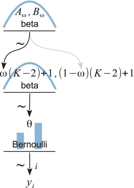
![]() ecall also, from Equation 6.6 (p. 129), that the shape parameters of the beta density, a and b, can be re-expressed in terms of the mode ω and concentration κ of the beta distribution: a = ω(k − 2) + 1 and b = (1 − ω)(κ − 2) +1, where ω = (a − 1)/(a + b − 2) and κ = a + b. Therefore Equation 9.3 can be re-expressed as
ecall also, from Equation 6.6 (p. 129), that the shape parameters of the beta density, a and b, can be re-expressed in terms of the mode ω and concentration κ of the beta distribution: a = ω(k − 2) + 1 and b = (1 − ω)(κ − 2) +1, where ω = (a − 1)/(a + b − 2) and κ = a + b. Therefore Equation 9.3 can be re-expressed as
Think for a moment about the meaning of Equation 9.4. It says that the value of θ depends on the value of ω. When ω is, say, 0.25, then θ will be near 0.25. The value of κ governs how near θ is to θ, with larger values of κ generating values of θ more concentrated near ω. Thus, the magnitude of κ is an expression of our prior certainty regarding the dependence of θ on ω. For the purposes of the present example, we will treat κ as a constant, and denote it as K.
Now we make the essential expansion of our scenario into the realm of hierarchical models. Instead of thinking of ω as fixed by prior knowledge, we think of it as another parameter to be estimated. Because of the manufacturing process, the coins from the minttend to have a bias near ω. Some coins randomly have a value of θ greater than ω, and other coins randomly have a value of θ less than ω. The larger K is, the more consistently the mint makes coins with θ close to ω. Now suppose we flip a coin from the mint and observe a certain number of heads and tails. From the data, we can estimate the bias θ of the coin, and we can also estimate the tendency ω of the mint. The estimated credible values of θ will (typically) be near the proportion of heads observed. The estimated credible values of ω will be similar to θ if K is large, but will be much less certain if K is small.
To infer a posterior distribution over ω, we must supply a prior distribution. Our prior distribution over ω expresses what we believe about how mints are constructed. For the sake of simplicity, we suppose that the prior distribution on ω is a beta distribution,
where Aω and Bω are constants. In this case, we believe that ω is typically near (Aω − 1)/ (Aω + Bω − 2), because that is the mode of the beta distribution.
The scenario is summarized in Figure 9.1. The figure shows the dependency structure among the variables. Downward pointing arrows denote how higher-level variables generate lower-level variables. For example, because the coin bias θ governs the result of a coin flip, we draw an arrow from the θ-parameterized Bernoulli distribution to the datum yi. As was emphasized in Section 8.2 in the discussion of Figure 8.2 (p. 196), these sorts of diagrams are useful for two reasons. First, they make the structure of the model visually explicit, so it is easy to mentally navigate the meaning of the model. Second, they facilitate expressing the model in JAGS (or Stan) because every arrow in the diagram has a corresponding line of code in the JAGS model specification.
Let's now consider how Bayes' rule applies to this situation. If we treat this situation as simply a case of two parameters, then Bayes' rule is merely p(θ,ω | y) = p(y | θ,ω)p(θ,ω)/p(y). There are two aspects that are special about our present situation. First, the likelihood function does not involve ω, so p(y | θ, ω) can be rewritten as p(y | θ). Second, because by definition p(θ | ω) = p(θ,ω)/p(ω), the prior on the joint parameter space can be factored thus: p(θ, ω) = p(θ | ω) p(ω). Therefore, Bayes' rule for our current hierarchical model has the form

Notice in the second line that the three terms of the numerator are given specific expression by our particular example The likelihood function, p(y | θ), is a Bernoulli distribution in Equation 9.2. The dependence of θ on ω, p(θ | ω), is specified to be a beta density in Equation 9.4. And the prior distribution on ω, p(ω),is defined to be a beta density in Equation 9.5. These specific forms are summarized in Figure 9.1. Thus, the generic expression in the first line of Equation 9.6 gains specific hierarchical meaning because of its factorization in the second line.
The concept expressed by Equation 9.6 is important. In general, we are merely doing Bayesian inference on a joint parameter space. But sometimes, as in this case, the likelihood and prior can be re-expressed as a hierarchical chain of dependencies among parameters. There are two reasons this is important. First, the semantics of the model matter for human interpretation, because the hierarchy is meaningful. Second, hierarchical models can sometimes be parsed for MCMC samplers very effectively. The algorithms in JAGS, for example, look for particular model substructures to which specific samplers can be applied.
Whether or not a model structure can be factored into a chain of hierarchical dependencies depends on the model's parameterization. Under some parameterizations there may be a natural factorization of dependencies, but under another parameterization there might not be. In typical applications of hierarchical models, the meaningful chain of dependencies is primary in the conceptual genesis of the model, and thinking of the model as a joint distribution on a joint parameter space is secondary.
9.1.1 Posterior via grid approximation
It turns out that direct formal analysis of Equation 9.6 does not yield a simple formula for the posterior distribution. We can, nevertheless, use grid approximation to get a thorough picture of what is going on. When the parameters extend over a finite domain, and there are not too many of them, then we can approximate the posterior via grid approximation. In our present situation, we have the parameters θ and ω that both have finite domains, namely the interval [0,1]. Therefore, a grid approximation is tractable and the distributions can be readily graphed.
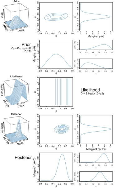
Figure 9.2 shows an example in which the prior distribution has Aω = 2, Bω = 2, and K = 100. The left and middle panels of the top row of Figure 9.2 show the joint prior distribution: p(θ,ω) = p(θ | ω)p(ω) = beta(θ| ω(100 − 2) + 1, (1 − ω)(100 − 2)+1) beta(ω | 2, 2). The contour plot in the middle panel shows a top-down view of the perspective plot in the left panel. As this is a grid approximation, the joint prior p(θ, ω) was computed by first multiplyingp(θ | ω) and p(ω) at every grid point and then dividing by their sum across the entire grid. The normalized probability masses were then converted to estimates of probability density at each grid point by dividing each probability mass by the area of a grid cell.

The right panel of the top row (Figure 9.2), showing p(ω) tipped on its side, is a “marginal” distribution of the prior: if you imagine collapsing (i.e., summing) the joint prior across θ, the resulting pressed flower2 is the graph of p(ω). The scale on the p(ω) axis is density, not mass, because the mass at each interval of the comb on ω was divided by the width of the interval to approximate density.
The implied marginal prior on θ is shown in the second row of Figure 9.2. It was computed numerically by collapsing the joint prior across ω. But notice, we did not explicitly formulate the marginal prior on θ. Instead, we formulated the dependence of θ on ω. The dependence is shown in the right panel of the second row, which plots p(θ | ω) for two values of ω. Each plot is a “slice” through the joint prior at a particular value of ω. The slices are renormalized, however, so that they are individually proper probability densities that sum to 1.0 over θ. One slice is p(θ | ω = 0.75), and the other slice is p(θ | ω = 0.25). You can see that the prior puts most credibility on θ values near ω. In fact, the slices are beta densities: beta(θ |(0.75)(100 − 2) +1, (1 − 0.75)(100 − 2) + 1) = beta(θ | 74.5,25.5) and beta(θ |(0.25)(100 − 2) + 1, (1 − 0.25)(100 − 2) + 1) = beta(θ | 25.5,74.5).
The likelihood function is shown in the middle row of Figure 9.2. The data comprise nine heads and three tails. The likelihood distribution is a product of Bernoulli distributions, p({ yi } | θ) = θ)= θ9(1 − θ)3. Notice in the graph that all the contour lines are parallel to the ω axis, and orthogonal to the θ axis. These parallel contours are the graphical signature of the fact that the likelihood function depends only on θ and not on ω.
The posterior distribution in the fourth row of Figure 9.2 is determined by multiplying, at each point of the grid on y, ω space, the joint prior and the likelihood. The point-wise products are normalized by dividing the sum of those values across the parameter space.
When we take a slice through the joint posterior at a particular value of ω, and renormalize by dividing the sum of discrete probability masses in that slice, we get the conditional distribution p(θ | ω, D). The bottom right panel of Figure 9.2 shows the conditional for two values of ω. Notice in Figure 9.2 that there is not much difference in the graphs of the prior p(θ | ω) and the posterior p(θ | ω, { yi}). This is because the prior beliefs regarding the dependency of θ on ω had little uncertainty.
The distribution of p(ω | { yi }), shown in the right panel of the fourth row of Figure 9.2, is determined by summing the joint posterior across all values of θ. This marginal distribution can be imagined as collapsing the joint posterior along the θ axis, with the resulting pressed flower being silhouetted in the third panel of the bottom row. Notice that the graphs of the prior p(ω) and the posterior p(ω | { yi }) are rather different. The data have had a noticeable impact on beliefs about how ω is distributed because the prior was very uncertain and was therefore easily influenced by the data.
As a contrasting case, consider instead what happens when there is high prior certainty regarding ω, but low prior certainty regarding the dependence of θ on ω. Figure 9.3 illustrates such a case, where Aω = 20, Bω = 20, and K = 6. The joint prior distribution is shown in the top row of Figure 9.3, left and middle panels. The marginal prior on ω is shown in the top row, right panel, where it can be seen that p(ω) is fairly sharply peaked over ω= 0.5. However, the conditional distributions p(θ | ω) are very broad, as can be seen in right panel of the second row.
The same data as for Figure 9.2 are used here, so the likelihood graphs look the same in the two figures. Notice again that the contour lines of the likelihood function are parallel to the ω axis, indicating that ω has no influence on the likelihood.
The posterior distribution is shown in the lower two rows of Figure 9.3. Consider the marginal posterior distribution on ω. Notice it has changed fairly little from the prior, because the distribution began with high certainty. Consider now the conditional posterior distributions in the lower right panels. They are very different from their priors,because they began with low certainty, and therefore the data can have a big impact on these distributions. In this case, the data suggest that θ depends on ω in a rather different way than we initially suspected. For example, even when ω = 0.25, the conditional posterior puts the most credible value of θ up near 0.6, not near 0.25.
In summary, Bayesian inference in a hierarchical model is merely Bayesian inference on a joint parameter space, but we look at the joint distribution (e.g., p(θ, ω))in terms of its marginal on a subset of parameters (e.g., p(ω)) and its conditional distribution for other parameters (e.g., p(θ |ω)). We do this primarily because it is meaningful in the context of particular models. The examples in Figures 9.2 and 9.3 graphically illustrated the joint, marginal, and conditional distributions. Those examples also illustrated how Bayesian inference has its greatest impact on aspects of the prior distribution that are least certain. In Figure 9.2, there was low prior certainty on ω (because Aω and Bω were small) but high prior certainty about the dependence of θ on ω (because K was large). The posterior distribution showed a big change in beliefs about γ, but not much change in beliefs about the dependence of θ on ω. Figure 9.3 showed the complementary situation, with high prior certainty on ω and low prior certainty about the dependence of θ on ω.
The aim of this section has been to illustrate the essential ideas of hierarchical models in a minimalist, two-parameter model, so that all the ideas could be graphically illustrated. While useful for gaining an understanding of the ideas, this simple, contrived example is also unrealistic. In subsequent sections, we progressively build more complex and realistic models.
9.2 Multiple coins from a single mint
The previous section considered a scenario in which we flip a single coin and make inferences about the bias θ of the coin and the parameter ω of the mint. Now we consider an interesting extension: what if we collect data from more than one coin created by the mint? If each coin has its own distinct bias θs, then we are estimating a distinct parameter value for each coin, and using all the data to estimate ω.
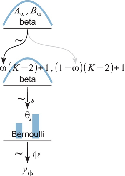
This sort of situation arises in real research. Consider, for example, a drug that is supposed to affect memory. The researcher gives the drug to several people, and gives each person a memory test, in which the person tries to remember a list of words. Each word is remembered or not (i.e., a dichotomous measurement). In this application, each person plays the role of a coin, whose probability of remembering a word is dependent on the tendency induced by the drug. Let's index the subjects in the experiment by the letter s. Then the probability of remembering by subject s is denoted θs. We assume that there is some random variation of subjects around the drug-induced tendency denoted as ω. In particular, we model the subjects' variation around ω as θs ~ dbeta(ω (K − 2) + 1, (1 − ω)(K − 2) + 1),where K is a fixed constant for now. We also assume that the performance of each subject depends only on that subject's individual θs, which is modeled as yi | s ~ dbern(θs), where the subscript, i | s, indicates the ith observation within subject s. The scenario is summarized in Figure 9.4. It is very much like Figure 9.1, but with changes on the subscripts to indicate multiple subjects. Notice that the model involves more than two parameters. If there are S subjects altogether, then there are S +1 parameters (namely θ1,…, θs, and ω) being estimated simultaneously. If our primary research interest is the overall effect of the drug, not the reactions of individual subjects, then we are most interested in the estimate of ω.
9.2.1 Posterior via grid approximation
As a concrete example, suppose we have only two subjects in the same condition (i.e., two coins from the same mint). We want to estimate the biases θ1 and θ2 of the two subjects, and simultaneously estimate ω of the drug that influenced them. Figures 9.5 and 9.6 show grid approximations for two different choices of prior distributions.
For the case illustrated in Figure 9.5, the prior on ω is gently peaked over ω = 0.5, in the form of a beta(ω | 2,2) distribution; that is, AωB=ω = 2 in the top-level formula of Figure 9.4. The biases of the coins are only weakly dependent on ω according to the prior p(θj | ω) = beta(θj | ω (5 − 2) + 1, (1 − ω)(5 − 2) + 1); that is, K = 5 in the middle-level formula of Figure 9.4.

The full prior distribution is a joint distribution over three parameters: ω, θ1, and θ2. In a grid approximation, the prior is specified as a three-dimensional (3D) array that holds the prior probability at various grid points in the 3D space. The prior probability at point 〈ω,θ1, θ2〉 is p(θ1 | ω) · p(θ2 | ω) · p(ω) with exact normalization enforced by summing across the entire grid and dividing by the total.
Because the parameter space is 3D, a distribution on it cannot easily be displayed on a 2D page. Instead, Figure 9.5 shows various marginal distributions. The top row shows two contour plots: one is the marginal distribution p(θ1ω) which collapses across θ2, and the other is the marginal distribution p(θ2ω) which collapses across θ1. From these contour plots you can see the weak dependence of θs on ω. The upper-right panel shows the marginal prior distribution p(ω), which collapses across θ1 and θ2. You can see that the marginal on p(ω) does indeed have the shape of a beta(2,2) distribution (but the p(ω) axis is scaled for probability masses at the arbitrary grid points, not for density).
The middle row of Figure 9.5 shows the likelihood function for the data, which comprise 3 heads out of 15 flips of the first coin, and four heads out of five flips of the second coin. Notice that the contours of the likelihood plot are parallel to the ω axis, indicating that the likelihood does not depend on ω. Notice that the contours are more tightly grouped for the first coin than for the second, which reflects the fact that we have more data from the first coin (i.e., 15 flips v. 5 flips).
The lower two rows of Figure 9.5 show the posterior distribution. Notice that the marginal posterior on θ1 is centered near the proportion 3/15 = 0.2 in its subject's data, and the posterior on θ2 is centered near the proportion 4/5 = 0.8 in its subject's data. The marginal posterior on θ1 has less uncertainty than the marginal posterior on θ2, as indicated by the widths of the distributions. Notice also that the marginal posterior on ω, at the right of the fourth row, remains fairly broad.
That result should be contrasted with the result in Figure 9.6, which uses the same data with a different prior. In Figure 9.6, the prior on ω is the same gentle peak, but the prior dependency of θs on ω is much stronger, with K = 75 instead of K = 5. The dependency can be seen graphically in the top two panels of Figure 9.6, which show contour plots of the marginals p(θs, ω). The contours reveal that the distribution of θs is tightly linked to the value of ω, along a ridge or spindle in the joint parameter space.

The plots of the posterior distribution, in the lower rows of Figure 9.6, reveal some interesting results. Because the biases θs are strongly dependent on the parameter ω, the posterior estimates are fairly tightly constrained to be near the estimated value of ω. Essentially, because the prior emphasizes a relatively narrow spindle in the joint parameter space, the posterior is restricted to a zone within that spindle. Not only does this cause the posterior to be relatively peaked on all the parameters, it also pulls all the estimates in toward the focal zone. Notice, in particular, that the posterior on θ2 is peaked around 0.4, far from the proportion 4/5 = 0.8 in its coin's data! This shift away from the data proportion of subject 2 is caused by the fact that the other coin had a larger sample size, and therefore had more influence on the estimate of ω, which in turn influenced the estimate of θ2. Of course, the data from subject 2 also influenced ω and θ1, but with less strength.
One of the desirable aspects of using grid approximation to determine the posterior is that we do not require any analytical derivation of formulas. Instead, our computer simply keeps track of the values of the prior and likelihood at a large number of grid points and sums over them to determine the denominator of Bayes' rule. Grid approximation can use mathematical expressions for the prior as a convenience for determining the prior values at all those thousands of grid points. What's nice is that we can use, for the prior, any (non-negative) mathematical function we want, without knowing how to formally normalize it, because it will be normalized by the grid approximation. My choice of the priors for this example, summarized in Figure 9.4, was motivated merely by the pedagogical goal of using functions that you are familiar with, not by any mathematical restriction.
The grid approximation displayed in Figures 9.5 and 9.6 used combs of only 50 points on each parameter (ω,θ1, and θ2). This means that the 3D grid had 503 = 125,000 points, which is a size that can be handled easily on an ordinary desktop computer of the early 21st century. It is interesting to remind ourselves that the grid approximation displayed in Figures 9.5 and 9.6 would have been on the edge of computability 50 years ago, and would have been impossible 100 years ago. The number of points in a grid approximation can get hefty in a hurry. If we were to expand the example by including a third coin, with its parameter θ3, then the grid would have 504 = 6,250,000 points, which already strains small computers. Include a fourth coin, and the grid contains over 312 million points. Grid approximation is not a viable approach to even modestly large problems, which we encounter next.
9.2.2 A realistic model with MCMC
The previous sections have used simplified hierarchical models for the purpose of being able to graphically display the distributions over parameter space and to gain clear intuitions about how Bayesian inference works. In this section, we will make the model realistic by including another parameter and including more subjects.
The previous examples arbitrarily fixed the degree of dependency of θ on ω. The degree of dependency was specified as the fixed value K of the concentration or consistency parameter, κ. When κ was fixed at a large value, then the individual θs values stayed close to ω, but when κ was fixed at a small value, then the individual θs values could roam quite far from ω.
In real situations, we do not know the value of κ in advance, and instead we let the data inform us regarding its credible values. Intuitively, when the data from different coins show very similar proportions of heads, we have evidence that κ is high. But when the data from different coins show diverse proportions of heads, then we have evidence that κ is small.
If we want to estimate a parameter, we must have prior uncertainty about it, otherwise we would not be trying to estimate it. If we want to estimate κ with Bayesian inference, we must formally express our prior uncertainty about it. Therefore, we expand the hierarchical model to include a prior distribution on κ, as shown in Figure 9.7. This model is just like the hierarchy of Figure 9.4, except that what was a constant K is now a parameter κ with its own prior distribution. Instead of specifying a single value of K, we allow a distribution of values κ.

Because the value of κ − 2 must be non-negative, the prior distribution on κ − 2 must not allow negative values. There are many distributions with this property, and we must use one that adequately expresses our prior knowledge. For our present application, we want the prior to be vague and noncommittal, allowing a broad range ofvalues for the concentration parameter. One distribution that is convenient for this purpose, because it is familiar in traditional mathematical statistics and available in JAGS (and in Stan and BUGS), is the gamma distribution. We will be using gamma distributions in a variety of contexts, just as we have been using beta distributions a lot.
The gamma(κ | s, r) distribution is a probability density for κ ≥ 0, with two parameters that determine its exact form, called its shape s and rate r parameters.3
Figure 9.8 shows examples of the gamma distribution with different values of the shape and rate parameters. The annotations in the panels of Figure 9.8 also show the corresponding mean, standard deviation, and mode of the distribution. The top-left panel shows a frequently used version in which both the shape and rate are set to equivalent small values. This setting results in the mean being 1 and the standard deviation being relatively large, with the mode at zero. The other three panels of Figure 9.8 show cases in which the mean is set to 50, but the standard deviations and modes differ. In the lower left, the standard deviation equals the mean, in which case the gamma distribution has shape = 1 (and is, in fact, an exponential distribution). In the right panels, the standard deviation is less than the mean, and you can see how the gamma distribution becomes less skewed as the standard deviation gets smaller, with the mode getting closer to the mean. I will use the generic shape of the upper-right panel of Figure 9.8 as the iconic gamma distribution in model diagrams such as Figure 9.7, because this shape suggests that the distribution has a left boundary of zero but an infinite extent on positive values.(Other distributions can have shapes that are visually similar, and therefore the icons are labeled with the name of the intended distribution.)

As you can see from Figure 9.8, it is not intuitively obvious how particular values of the shape and rate parameters correspond with particular visual shapes of the gamma distribution. Moreover, prior beliefs are most intuitively expressed in terms of the central tendency and a width of the distribution. Therefore, it would be useful to be able to start with values for central tendency and width, and convert them into corresponding shape and rate values. It turns out that the mean of the gamma distribution is μ = s/r, the mode is ω = (s − 1)/r for s > 1, and the standard deviation is ![]() . Algebraic manipulation then yields the following formulas for the shape and rate values in terms of the mean and standard deviation, or mode and standard deviation:
. Algebraic manipulation then yields the following formulas for the shape and rate values in terms of the mean and standard deviation, or mode and standard deviation:
For example, suppose we desire a gamma distribution with a mode of ω = 42 and a standard deviation of σ = 20. We compute the corresponding shape and rate from Equation 9.8, which yields ![]() and s = 1 + 42 · 0.125 = 6.25, as shown in the lower-right panel of Figure 9.8.
and s = 1 + 42 · 0.125 = 6.25, as shown in the lower-right panel of Figure 9.8.
I have created convenient utility functions in ![]() that implement the parameter transformations in Equations 9.7 and 9.8. The functions are loaded into
that implement the parameter transformations in Equations 9.7 and 9.8. The functions are loaded into ![]() by typing source(“DBDA2E-utilities.R”), when that file is in the current working directory. Hopefully the function names are self-explanatory, and here is an example of their use:
by typing source(“DBDA2E-utilities.R”), when that file is in the current working directory. Hopefully the function names are self-explanatory, and here is an example of their use:
The functions return a list of named components. Therefore, if you assign the result of the function to a variable, you can get at the individual parameters by their component names, as in the following example:
You may find those functions useful when you are setting the constants for prior distributions. If you want to graph a gamma distribution in R, the gamma density is provided by dgamma(x,shape=s,rate=r). As we will see in the next section, JAGS parameterizes the gamma distribution with shape and rate parameters in that order.
9.2.3 Doing it with JAGS
Look again at the hierarchical diagram in Figure 9.7 (p. 236). The arrows in that diagram indicate the dependencies between the variables. The key thing to understand is that every arrow in the hierarchical diagram has a corresponding expression in the JAGS model specification. The JAGS model specification is a verbal code for the graphical diagram. Here is a JAGS model specification that corresponds to Figure 9.7:
The beginning of the model specification expresses the arrow for the Bernoulli likelihood function and uses nested indexing in theta[s[i]], as was explained in Section 8.4 (p. 208). Moving up the diagram in Figure 9.7, the arrow expressing the prior on ω is coded in JAGS as omega ~ dbeta(1,1), which is a uniform distribution. In general, the prior on ω can be whatever is an appropriate description of real prior knowledge. In the present implementation, a vague and noncommittal prior is used for generic application.
Finally, the prior on κ − 2 is implemented by two lines of code in the JAGS model specification, repeated here:
Notice that the dgamma distribution generates a variable called kappaMinusTwo, and then kappa itself is kappaMinusTwo + 2. This two-line implementation is needed because the gamma distribution covers zero to infinity, but κ must be no smaller than 2. The choice of shape and rate constants in the dgamma distribution makes the prior allow avery broad range of κ values, yielding a sensible prior on θs as will be shown later. Exercise 9.1 explores different priors on κ.
These details of the model specification in JAGS have been presented to demonstrate how easy it is to implement a hierarchical model in JAGS. If you can draw a coherent hierarchical diagram, then you can implement it in JAGS. This functionality provides great flexibility for defining meaningful descriptive models of data. I have created scripts for using the model that require no knowledge of the implementation details, as explained in the following example.
9.2.4 Example: Therapeutic touch
Therapeutic touch is a nursing technique in which the practitioner manually manipulates the “energy field” of a patient who is suffering from a disease. The practitioner holds her or his hands near but not actually touching the patient, and repatterns the energy field to relieve congestion and restore balance, allowing the body to heal. Rosa, Rosa, Sarner, and Barrett (1998)reported that therapeutic touch has been widely taught and widely used in nursing colleges and hospitals despite there being little ifany evidence of its efficacy.
Rosa et al. (1998) investigated a key claim of practitioners of therapeutic touch, namely, that the practitioners can sense a body's energy field. If this is true, then practitioners should be able to sense which of their hands is near another person's hand, even without being able to see their hands. The practitioner sat with her hands extended through cutouts in a cardboard screen, which prevented the practitioner from seeing the experimenter. On each trial, the experimenter flipped a coin and held her hand a few centimeters above one or the other of the practitioner's hands, as dictated by the flip of the coin. The practitioner then responded with her best guess regarding which of her hand's was being hovered over. Each trial was scored as correct or wrong. The experimenter (and co-author of the article) was 9‒years old at the time.
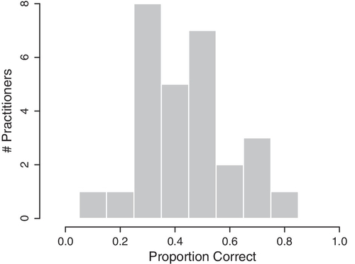
Each practitioner was tested for 10 trials. There were a total of 21 practitioners in the study, seven of whom were tested twice approximately a year apart. The retests were counted by the authors as separate subjects, yielding 28 nominal subjects. The proportions correct for the 28 subjects are shown in Figure 9.9. Chance performance is 0.50. The question is how much the group as a whole differed from chance performance, and how much any individuals differed from chance performance. The hierarchical model of Figure 9.7 is perfect for these data, because it estimates the underlying ability of each subject while simultaneously estimating the modal ability of the group and the consistency of the group. Moreover, the distribution of proportions correct across subjects (Figure 9.9) is essentially unimodal and can be meaningfully described as a beta distribution. With 28 subjects, there are a total of 30 parameters being estimated.
Below is a script for running the analysis on the therapeutic touch data. The script has a structure directly analogous to the scripts used previously, such as the one described in Section 8.3. The complete script is the file named Jags-Ydich- XnomSsubj-MbernBetaOmegaKappa-Example. R. Please read through the excerpt below, paying attention to the comments:
The data file must be arragnged with one column that contains the outcome of the trials (i.e., 0 or 1 in each row), and another column that contains the identifier of the subject who generated each outcome. The subject identifier could be a numerical integer or a character string. The first row of the data file must contain the names of the columns, and those column names are included as the arguments sName and yName in the functions genMCMC and plotMCMC. If you look at the file TherapeuticTouchData.csv, you will see that it has two columns, one column named “y” consisting of 0's and 1's, and a second column named “s” consisting of subject identifiers such as S01, S02, and so on. When the file is read by the read.csv function, the result is a data frame that has a vector named “y” and a factor named “s.”
In the call to the genMCMC function, you can see that there are 20,000 saved steps and thinning of 10 steps. These values were chosen after a short initial run with no thinning (i.e., thinSteps=1) showed strong autocorrelation that would have required a very long chain to achieve an effective sample size of 10,000 for the ω parameter. To keep the saved MCMC sample down to a modest file size (under 5 MB), I chose to set thinSteps=10 and to save 20,000 of the thinned steps. This still required waiting through 200,000 steps, however, and throwing away information. If computer memory is of no concern, then thinning is neither needed nor recommended. When you run the script, you will notice that it takes a minute for JAGS to generate the long chain. Section 9.4 discusses ways to speed up the processing.
The diagnostic plots produced by calls to the diagMCMC function all showed adequate convergence. They are not shown here, but you can see them by running the script yourself. Only the kappa parameter showed high autocorrelation, which is typical of higher-level parameters that control the variance of lower-level parameters. Nevertheless, the chains for κ show good overlap and we are not concerned with a very accurate estimate of its value. Moreover, we will see that the marginal posterior on κ spans a wide range of values, and the estimates of the other parameters are not hugely affected by small changes in κ.
A numerical summary of the posterior distribution is produced by the smryMCMC function. An argument of the function that is unique to this model is diffIdVec. It specifies a vector of subject indices that should have their posterior differences summarized. For example, diffIdVec=c(1,14,28) produces summaries of the posterior distributions of θ1 − θ14, θ1 − θ28, and θ14 − θ28. The argument defaults to showing no differences instead of all differences (which, in this application, would yield 28(28 − 1)/2 = 378 differences).
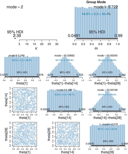
Finally, a graphical summary of the posterior distribution is produced by the plotMCMC function. It also has the diffldVec argument to specify which differences should be displayed. The result is shown in Figure 9.10. The posterior distribution reveals several interesting implications, described next.

The upper-right panel of Figure 9.10 shows the marginal posterior distribution on the group-level mode, ω. It's most credible value is less than 0.5, and its 95% HDI includes the chance value of 0.5, so we would certainly not want to conclude that the group of practitioners, as a class, detects the energy field of a nearby hand better than chance. (If the group mode had been credibly less than 0.5, we might have inferred that the practitioners as a group could detect the experimenter's hand but then systematically misinterpreted the energy field to give a contrary response.)
The lower three rows of Figure 9.10 show marginal posteriors for θs of selected individuals. The data conveniently ordered the subject identifiers so that subject 1 had the worst performance and subject 28 had the best performance, with the others between, such that subject 14 was near the 50th percentile of the group. Down the diagonal panels are the estimates of the individual parameters. You can see that the estimate for theta[1] has its peak around 0.4, even though this subject got only 1 out of 10 trials correct, as indicated by the “+” marked on the horizontal axis at 0.10. The estimate is pulled above the subject's actual performance because there are 27 other subjects all providing data that indicate typical performance is higher. In other words, the 27 other subjects inform the estimate of group-level parameters, and those group-level parameters pull the estimate of the individual toward what is typical for the group. The same phenomenon can be seen in the lower-right panel, where it can be seen the estimate for the best subject peaks around 0.5, even though this subject got 8 out of 10 trials correct, as shown by the “+” marked at 0.8 on the horizontal axis. The 95% HDI's of even the worst and best subjects include 0.5, so we cannot conclude that any of the subjects were performing credibly differently than chance.
The lower three rows of Figure 9.10 also show pairs of individual estimates and their differences. We might be interested, for example, in whether the worst and best subjects performed very differently. The answer is provided by the marginal posterior on the difference θ1 − θ28, plotted in the right column. The most credible difference is near −0.1 (which is nowhere near the difference of proportions exhibited by the subjects, indicated by the “+” on the horizontal axis), and the 95% HDI includes a difference of zero.
In conclusion, the posterior distribution indicates that the most credible values for the group as a whole and for all the individuals include chance performance. Either the experiment procedure was not appropriate for detecting the abilities of therapeutic touch practitioners, or much more data would be needed to detect a very subtle effect detectable by the procedure, or there is no actual sensing ability in the practitioners. Notice that these conclusions are tied to the particular descriptive model we used to analyze the data. We used a hierarchical model because it is a reasonable way to capture individual differences and group-level tendencies. The model assumed that all individuals were representative of the same overarching group, and therefore all individuals mutually informed each other's estimates.
It can be very useful to view the prior distribution in hierarchical models, as sometimes the prior on mid-level parameters, implied by the top-level prior, is not actually what was intuited or intended. It is easy to make JAGS produce an MCMC sample from the prior by running the analysis without the data, as was explained in Section 8.5 (p. 211).
The prior for the therapeutic touch data is shown in Figure 9.11. It can be seen that the prior is uniform on the group-level mode, ω, and uniform on each of the individual level biases, θs. This is good because it was what was intended, namely, to be noncommittal and to give equal prior credibility to any possible bias.4
The priors on the differences of individual biases are also shown in Figure 9.11. They are triangular distributions, peaked at a difference of zero. You can understand why this shape arises by examining the scatter plots of the joint distributions in the lower left. Those scatter plots are uniform across the two dimensions, so when they are collapsed along the diagonal that marks a difference of zero, you can see that there are many more points along the diagonal, and the number of points drops off linearly toward the corners. This triangular prior on the differences might not have been what you imagined it would be, but it is the natural consequence of independent uniform priors on the individual parameters. Nevertheless, the prior does show a modest preference for differences of zero between individuals.
9.3 Shrinkage in hierarchical models
In typical hierarchical models, the estimates of low-level parameters are pulled closer together than they would be if there were not a higher-level distribution. This pulling together is called shrinkage of the estimates. We have seen two cases of shrinkage, one in Figure 9.10 and another previously in Figure 9.6 (p. 234). In Figure 9.10, the most credible values of individual-level biases, θs, were closer to the group-level mode, ω,than the individual proportions correct, zs/Ns. Thus, the variance between the estimated values θs is less than the variance between the data values zs/Ns.
This reduction of variance in the estimators, relative to the data, is the general property referred to by the term “shrinkage.” But the term can be misleading because shrinkage leads to reduced variance only for unimodal distributions of parameters. In general, shrinkage in hierarchical models causes low-level parameters to shift toward the modes of the higher-level distribution. If the higher-level distribution has multiple modes, then the low-level parameter values cluster more tightly around those multiple modes, which might actually pull some low-level parameter estimates apart instead of together. Examples are presented at the book's blog (http://doingbayesiandataanalysis.blogspot.com/2013/03/shrinkage-in-bimodal-hierarchical.html) and in Kruschke and Vanpaemel (in press).
Shrinkage is a rational implication of hierarchical model structure, and is (usually) desired by the analyst because the shrunken parameter estimates are less affected by random sampling noise than estimates derived without hierarchical structure. Intuitively, shrinkage occurs because the estimate of each low-level parameter is influenced from two sources: (1) the subset of data that are directly dependent on the low-level parameter, and (2) thehigher-level parameters on which the low-level parameter depends. The higher-level parameters are affected by all the data, and therefore the estimate of a low-level parameter is affected indirectly by all the data, via their influence on the higher-level parameters.
It is important to understand that shrinkage is a consequence of hierarchical model structure, not Bayesian estimation. To better understand shrinkage in hierarchical models, we will consider the maximum likelihood estimate (MLE) for the hierarchical model of Figure 9.7. The MLE is the set of parameter values that maximizes the probability of the data. To find those values, we need the formula for the probability of the data, given the parameter values. For a single datum, yi | s, that formula is

For the whole set of data, {yi | s}, because we assume independence across data values, we take the product of that probability across all the data:
In that formula, remember that the yi | s values are constants, namely the 0's and 1's in the data. Our goal here is to find the values of the parameters in the formula that will maximize the probability of the data. You can see that ys participates in both the low-level data probability, ![]() , and in the high-level group probability, beta(θs | ω (κ − 2) +1, (1−ω)(κ−2)+1). The value of θs that maximizes the low-level data probability is the data proportion, zs/Ns. The value of θs that maximizes the high-level group probability is the higher-level mode, ω. The value of θs that maximizes the product of low-level and high-level falls between the data proportion, zs/Ns, and the higher-level mode, ω. In other words, θs is pulled toward the higher-level mode.
, and in the high-level group probability, beta(θs | ω (κ − 2) +1, (1−ω)(κ−2)+1). The value of θs that maximizes the low-level data probability is the data proportion, zs/Ns. The value of θs that maximizes the high-level group probability is the higher-level mode, ω. The value of θs that maximizes the product of low-level and high-level falls between the data proportion, zs/Ns, and the higher-level mode, ω. In other words, θs is pulled toward the higher-level mode.
As a concrete numerical example, suppose we have five individuals, each of whom went through 100 trials, and had success counts of 30, 40, 50, 60, and 70. It might seem reasonable that a good description of these data would be θ1 = z1N1 = 30/100 = 0.30, θ2 = z2N2 = 40/100 = 0.40, and so on, with a higher-level beta distribution that is nearly flat. This description is shown in the left panel of Figure 9.12. The probability of the data, given this choice of parameter values, is the likelihood computed from Equation 9.10 and is displayed at the top of the panel. Although this choice of parameter values is reasonable, we ask: are there other parameter values that increase the likelihood? The answer is yes, and the parameter values that maximize the likelihood are displayed in the right panel of Figure 9.12. Notice that the likelihood (shown at the top of the panel) has increased by a factor ofmore than 20. The θs values in the MLE are shrunken closer to the mode of the higher-level distribution, as emphasized by the arrows in the plot.

Intuitively, shrinkage occurs because the data from all individuals influence the higher-level distribution, which in turn influences the estimates of each individual. The estimate of θs is a compromise between the data zs/Ns of that individual and the group-level distribution informed by all the individuals. Mathematically, the compromise is expressed by having to jointly maximize ![]() and beta(θs | ω(κ − 2) +1, (1−ω)(κ−2)+1. The first term is maximized by θs = zs/Ns and the second term is maximized by θs = ω. As θs is pulled away from zs/Ns toward ω, the first term gets smaller but the second term gets larger. The MLE finds the best compromise between the two factors.
and beta(θs | ω(κ − 2) +1, (1−ω)(κ−2)+1. The first term is maximized by θs = zs/Ns and the second term is maximized by θs = ω. As θs is pulled away from zs/Ns toward ω, the first term gets smaller but the second term gets larger. The MLE finds the best compromise between the two factors.
In summary, shrinkage is caused by hierarchical structure. We have seen how shrinkage occurs for the MLE. The MLE involves no prior on the top-level parameters,of course. When we use Bayesian estimation, we supply a prior distribution on the top-level parameters, and infer an entire posterior distribution across the joint parameter space. The posterior distribution explicitly reveals the parameter values that are credible and their uncertainty, given the data. Exercise 9.3 explores the Bayesian analysis of the data in Figure 9.12.
9.4 Speeding up jags
In this section, we consider two ways to speed up processing of JAGS. One method changes the likelihood function in the JAGS model specification. A second method uses the runjags package to run chains in parallel on multicore computers. The two methods are discussed in turn.
When there are many trials per subject, generating the chains in JAGS can become time consuming. One reason for slowness is that the model specification (recall Section 9.2.3) tells JAGS to compute the Bernoulli likelihood for every single trial:
Although that statement (above) looks like a for-loop in ![]() that would be run in a sequential procedure, it is really just telling to JAGS to set up many copies of the Bernoulli relation. Even though JAGS is not cycling sequentially through the copies, there is extra computational overhead involved. It would be nice if, instead of evaluating a Bernoulli distribution Ns times, we could tell JAGS to compute
that would be run in a sequential procedure, it is really just telling to JAGS to set up many copies of the Bernoulli relation. Even though JAGS is not cycling sequentially through the copies, there is extra computational overhead involved. It would be nice if, instead of evaluating a Bernoulli distribution Ns times, we could tell JAGS to compute ![]() just once.
just once.
We can accomplish this by using the binomial likelihood function instead of the Bernoulli likelihood. The binomial likelihood is ![]() ,where
,where ![]() is a constant called the binomial coefficient. It will be explained later, accompanying Equation 11.5 on p. 303, but for now all you need to know is that it is a constant. Therefore, when the binomial likelihood is put into Bayes' rule, the constant appears in the numerator and in the denominator and consequently cancels out, having no influence. Thus, we “trick” JAGS into computing
is a constant called the binomial coefficient. It will be explained later, accompanying Equation 11.5 on p. 303, but for now all you need to know is that it is a constant. Therefore, when the binomial likelihood is put into Bayes' rule, the constant appears in the numerator and in the denominator and consequently cancels out, having no influence. Thus, we “trick” JAGS into computing ![]() by using its built-in binomial likelihood.5
by using its built-in binomial likelihood.5
The necessary changes in the program are simple and few. First, we compute the zs and Ns values from the data. The code below assumes that y is a vector of 0's and 1's, and that s is vector of integer subject identifiers. The code uses the aggregate function, which was explained in Section 3.6.
Notice that the dataList (above) no longer includes any mention of y or Ntotal. The only information sent to JAGS is zs, Ns, and the overall number of subjects, Nsubj.
Then we modify the model specification so it uses the binomial distribution, which is called dbin in JAGS:
The only change in the model specification (above) was removing the loop for y[i]~dbern(theta[s[i]]) and putting the new binomial likelihood inside the subject loop.
The changes described above have been implemented in programs with file names beginning with Jags-Ydich-XnomSsubj-MbinomBetaOmegaKappa. Notice in the file name that the part starting with “-M”says binom instead of bern. Notice also that the part starting with “-Y”still says dich because the data are still dichotomous 0's and 1's, only being converted internally to z's and N's for computational purposes. To run the binomial version, all you have to do is tell ![]() to load it instead of the Bernoulli version:
to load it instead of the Bernoulli version:
For the modest amount of data in the therapeutic-touch experiment, the acceleration achieved by using the binomial instead of the Bernoulli is slight. But for larger data sets, the reduction in duration can be noticeable. The duration of the MCMC sampling can be measured in ![]() using the proc.time function that was explained in Section 3.7.5, p. 66. Exercise 9.4 shows an example.
using the proc.time function that was explained in Section 3.7.5, p. 66. Exercise 9.4 shows an example.
An important way to speed the processing of the MCMC is to run them in parallel with the runjags package, as was explained in Section 8.7, p. 215. The program Jags-Ydich-XnomSsubj-MbinomBetaOmegaKappa.R has been set up with runjags with parallel chains as its default. You can alter the setting inside the program, then save the program and re-source it, and then see how much slower it runs in nonparallel mode. I have found that it takes about half the time to run with three parallel chains as for one long chain, achieving about the same ESS either way. Exercise 9.4 provides more prompts for you to try this yourself.
9.5 Extending the hierarchy: Subjects within categories
Many data structures invite hierarchical descriptions that may have multiple levels. Software such as JAGS makes it easy to implement hierarchical models, and Bayesian inference makes it easy to interpret the parameter estimates, even for complex nonlinear hierarchical models. Here, we take a look at one type of extended hierarchical model.
Suppose our data consist of many dichotomous values for individual subjects from different categories, with all the categories under an overarching common distribution. For example, consider professional baseball players who, over the course of a year of games, have many opportunities at bat, and who sometimes get a hit. Players have different fielding positions (e.g., pitcher, catcher, and first base), with different specialized skills, so it is meaningful to categorize players by their primary position. Thus, we estimate batting abilities for individual players, and for positions, and for the overarching group of professional players. You may be able to think of a number of analogous structures from other domains.
This sort of hierarchical model structure is depicted in Figure 9.13. It is the same as the diagram in Figure 9.7 but with an extra layer added for the category level, along with the subscripts needed to indicate the categories. At the bottom of Figure 9.13, the individual trials are denoted as yi | s,c to indicate instances within subjects s and categories c. The underlying bias of subject s within category c is denoted θs | c. The biases of subjects within category c are assumed to be distributed as a beta density with mode ωc and concentration κc. Thus, each category has its own modal bias ωc, from which all subject biases in the category are assumed to be drawn. Moving up the diagram, the model assumes that all the category modes come from a higher-level beta distribution that describes the variation across categories. The modal bias across categories is denoted ω (without a subscript), and the concentration of the category biases is denoted κ (without a subscript). When κ is large, the category biases ωc are tightly concentrated. Because we are estimating ω and κ, we must specify prior distributions for them, indicated at the top of the diagram.
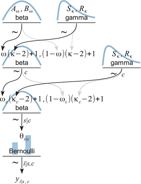
This model has an over-arching distribution over the category modes, ωc, that has its central tendency ω and scale κ estimated. But, purely for simplicity, the model does not have an over-arching distribution on the category concentrations κc that has its central tendency and scale estimated. In other words, the prior on κc applies independently to each κc in a manner fixed by the prior constants Sκ and Rκ ,and the κc's do not mutually inform each other via that part of the hierarchy. The model could be extended to include such an overarching distribution, as was done in a version on the book's blog (http://doingbayesiandataanalysis.blogspot.com/2012/11/shrinkage-in-multi-level-hierarchical.html).
Whereas the data are really 0's and 1's from individual trials, we will assume the data file has total results for each subject, and is arranged with one row per subject, with each row indicating the number of successes (or heads), zs | c, the number of attempts (or flips), Ns | c, and the category of the subject, c. Each row could also contain a unique subject identifier for ease of reference. The categories could be indicated by meaningful textual labels, but we will assume that they are converted by the program into consecutive integers for indexing purposes. Therefore, in the JAGS code below, we will use the notation c[s] for the integer category label of subject s.
Expressing the hierarchical model of Figure 9.13 in JAGS is straight forward. For every arrow in the diagram, there is a corresponding line of code in the JAGS model specification:
Because the data have been totaled, the expression of the likelihood uses a binomial (dbin) instead of Bernoulli distribution, without looping over trials i, as was explained previously in Section 9.4. Notice the nested indexing for categories in omega[c[s]], whichuses the mode of the appropriate categoryfordescribingthe individual theta[s]. The overarching ω and κ (with no subscript) in Figure 9.13 are coded as omega0 and kappa0.
This example is intended to demonstrate how easy it is to specify a complex hierarchical model in JAGS. If you can make a coherent model diagram for whatever application you are considering, then you can probably implement that model in JAGS. In fact, that is the method I use when I am building a new JAGS program: I start by making a diagram to be sure I fully understand the descriptive model, then I create the JAGS code arrow by arrow, starting at the bottom of the diagram. In the next section, we consider a specific application and see the richness of the information produced by Bayesian inference.
9.5.1 Example: Baseball batting abilities by position
Consider the sport of baseball. During a year of games, different players have different numbers of opportunities at bat, and on some of these opportunities a player might actually hit the ball. In American Major League Baseball, the ball is pitched very fast, sometimes at speeds exceeding 90 miles (145 km) per hour, and batters typically hit the ball on about only 23% of their opportunities at bat. That ratio, of hits divided by opportunities at bat, is called the batting average of each player. We can think of it as an indicator of the underlying probability that the player will hit the ball for any opportunity at bat. We would like to estimate that underlying probability, as one indicator of a player's ability. Players also must play a position in the field when the other team is at bat. Different fielding positions have different specialized skills, and those players are expected to focus on those skills, not necessarily on hitting. In particular, pitchers typically are not expected to be strong hitters, and catchers might also not be expected to focus so much on hitting. Most players have a primary fielding position, although many players perform different fielding positions at different times. For purposes of simplifying the present example, we will categorize each player into a single primary fielding position.
If you, like me, are not a big sports fan and do not really care about the ability of some guy to hit a ball with a stick, then translate the situation into something you do care about. Instead of opportunities at bat, think of opportunities to cure a disease, for treatments categorized into types. We are interested in estimating the probability of cure for each treatment and each type of treatment and overall across treatments. Or think of opportunities for students to graduate from high school, with schools categorized by districts. We are interested in estimating the probability of graduation for each school and each district and overall. Or, if that's boring for you, keep thinking about guys swinging sticks.
The data consist of records from 948 players in the 2012 regular season of Major League Baseball.6 For player s, we have his (it was an all-male league) number of opportunities at bat, Ns | c, his number of hits, zs | c and his primary position when in the field, cs, which was one of nine possibilities (e.g., pitcher, catcher, and first base). All players for whom there were zero at-bats were excluded from the data set. To give some sense of the data, there were 324 pitchers with a median of 4.0 at-bats, 103 catchers with a median of 170.0 at-bats, and 60 right fielders with a median of 340.5 at-bats, along with 461 players in six other positions. As you can guess from these data, pitchers are not of ten at bat because they are prized for their pitching abilities not necessarily for their batting abilities.
The CSV data file is named BattingAverage.csv and looks like this:
The first line (above) is the column names. Notice that there are six columns. The first four columns are the player's name (Player), primary position (PriPos), hits (Hits), and at-bats (AtBats). The last two columns are redundant numerical recodings of the player name and primary position; these columns will not be used in our analysis and could be completely omitted from the data file.
A script for analyzing the data follows the same sequence of steps as previous scripts, and looks like this:
Notice that the name of the function-definition file includes “Ybinom” because the data file codes the data as z and N, and the file name includes “XnomSsubjCcat” because both subject and category identifiers are used as predictors. There are a few arguments in the function calls that are specific to this form of data and model. In particular, we have to tell the functions which columns of the data frame correspond to the variables zs | c, Ns | c, s, and c. For example, the argument zName=“Hits” indicates that the column name of the zs| c data is Hits, and the argument cName=“PriPos” indicates that the column name of the category labels is PriPos.
The genMCMC command indicates that JAGS should save 11,000 steps thinned by 20. These values were chosen after an initial short run showed fairly high autocorrelation.
The goal was to have an effective sample size (ESS) of at least 10,000 for the key parameters (and differences of parameters) such as θs and ωc, while also keeping the saved file size as small as possible. With 968 parameters, 11,000 steps takes more than 77 MB of computer memory. The genMCMC function uses three parallel chains in runjags by default, but you can change that by altering the innards of the genMCMC function. Even when using three parallel chains, it takes about 11 min to run on my modest desktop computer (plus additional time for making diagnostic graphs, etc.).
The last command in the script, plotMCMC, uses new arguments diffCList and diffSList. These arguments take lists of vectors that indicate which specific categories or subjects you want to compare. The example above produces plots of the marginal posterior of the difference between the modes for category Pitcher and category Catcher, and for subjects Kyle Blanks versus Bruce Chen, etc. The plots are shown in figures described next.
JAGS produces combinations of parameter values in the 968-dimensional parameter space that are jointly credible, given the data. We could look at the results many different ways, based on whatever question we might ponder. For every pair of players, we could ask how much their estimated batting abilities differ. For every pair of positions, we can ask how much their batting abilities differ. (We could also ask questions about combinations of positions, such as, Do outfielders have different batting averages than basemen? But we will not pursue that sort of question here.) Selected illustrative results are shown in Figures 9.14–9.16. (We cannot get a sense of the difference of two parameters merely by looking at the marginal distributions of those parameters, as will be explained in Section 12.1.2.1, p. 340.)
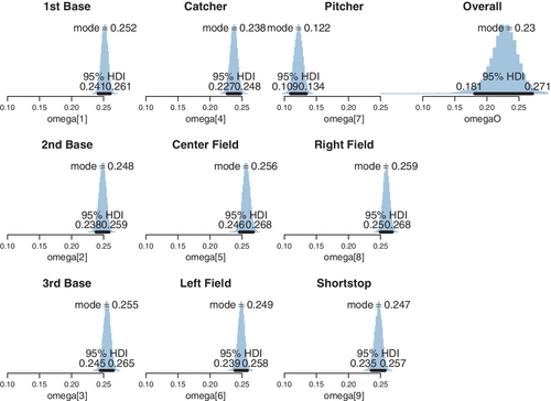
Figure 9.14 shows estimates of position-level batting abilities (the ωc parameters in the model). Clearly the modal batting ability of pitchers is lower than that of catchers. The modal ability of catchers is slightly lower than that of first-base men. Because the individual-level parameters (θs | c) are modeled as coming from position-specific modes, the individual estimates are shrunken toward the position-specific modes.

Figure 9.15 shows estimated abilities of selected individuals. The left panel shows two players with identical batting records but with very different estimated batting abilities because they play different positions. These two players happened to have very few opportunities at bat, and therefore their estimated abilities are dominated by the position information. This makes sense because if all we knew about the players was their positions, then our best guess would come from what we knew about other players from those positions. Notice that if we did not incorporate position information into our hierarchical model, and instead put all 948 players under a single over-arching distribution, then the estimates for two players with identical batting records would be identical regardless of the position they play.

The right panel of Figure 9.15 shows estimated abilities of two right fielders with many at-bats (and very strong batting records). Notice that the widths of their 95% HDIs are smaller than those in the left panel because these players have so much more data. Despite the large amount of data contributing to the individual estimates, there is still noticeable shrinkage of the estimates away from the proportion of hits (marked by the “+” signs on the horizontal axis) toward the modal value of all right fielders, which is about 0.247. The difference between the estimated abilities of these two players is centered almost exactly on zero, with the 95% HDI of the difference essentially falling within a ROPE of −0.04 to +0.04.
Figure 9.16 shows two comparisons of players from the same positions but with very different batting records. The left panel shows two pitchers, each with a modest number of at-bats. Despite the very different proportions of hits attained by these players, the posterior estimate of the difference of their abilities only marginally excludes zero because shrinkage pulls their individual estimates toward the mode of pitchers. The right panel shows two center fielders, one of whom has a large number of at-bats and an exceptional batting record. Because of the large amount of data from these individuals, the posterior distribution of the difference excludes zero despite within-position shrinkage.

This application was initially presented at the book's blog (http://doingbayesiandataanalysis.blogspot.com/2012/11/shrinkage-in-multi-level-hierarchical.html) and subsequently described by Kruschke and Vanpaemel (in press). In those reports, the models parameterized the beta distributions by means instead of by modes, and the models also put an estimated higher-level distribution on the κc parameters, instead of using a fixed prior. Despite those differences, they came to similar conclusions as those shown here.
Summary of example. This example has illustrated many important concepts in hierarchical modeling that are recapitulated and amplified in the following paragraphs.
The example has dramatically illustrated the phenomenon of shrinkage in hierarchical models. In particular, we saw shrinkage of individual-ability estimates based on category (fielding position). Because there were so many players contributing to each position, the position information had strong influence on the individual estimates. Players with many at-bats (large Ns) had somewhat less shrinkage of their individual estimates than players with few at-bats (small Ns), who had estimates dominated by the position information.
Why should we model the data with hierarchical categories at all? Why not simply put all 948 players under one group, namely, major-leaguers, instead of in nine subcategories within major leaguers? Answer: the hierarchical structure is an expression of how you think the data should be meaningfully modeled, and the model description captures aspects of the data that you care about. If we did not categorize by position, then the estimated abilities of the pitchers would be much more noticeably pulled up toward the modal abilities of all the nonpitchers. And, if we did not categorize by position, then the estimated abilities of any two players with identical batting records would also be identical regardless of their positions; for example, the first-base man and pitcher in Figure 9.15 would have identical estimates. But if you think that position information is relevant for capturing meaningful aspects of the data, then you should categorize by position. Neither model is a uniquely “correct” description of the data. Instead, like all models, the parameter estimates are meaningful descriptions of the data only in the context of the model structure.
An important characteristic of hierarchical estimation that has not yet been discussed is illustrated in Figure 9.17. The certainty of the estimate at a level in the hierarchy depends (in part) on how many parameter values are contributing to that level. In the present application, there are nine position parameters (ωc) contributing to the overall mode (ω), but dozens or hundreds of players contributing to each position (ωc). Therefore, the certainty of estimate at the overall level is less than the certainty of estimate within each position. You can see this in Figure 9.17 by the widths of the 95% HDIs. At the overall level, the 95% HDI on ω has a width of about 0.09. But for the specific positions, the 95% HDI on ωc has a width of about only 0.02. Other aspects of the data contribute to the widths and shapes of the marginal posterior distributions at the different levels, but one implication is this: if there are only a few categories, the overall level typically is not estimated very precisely. Hierarchical structure across categories works best when there are many categories to inform the higher-level parameters.
Finally, we have only looked at a tiny fraction of the relations among the 968 parameters. We could investigate many more comparisons among parameters if we were specifically interested. In traditional statistical testing based on p-values (which will be discussed in Chapter 11), we would pay a penalty for even intending to make more comparisons. This is because a p value depends on the space of counter-factual possibilities created from the testing intentions. In a Bayesian analysis, however, decisions are based on the posterior distribution, which is based only on the data (and the prior), not on the testing intention. More discussion of multiple comparisons can be found in Section 11.4.
9.6 Exercises
Look for more exercises at https://sites.google.com/site/doingbayesiandataanalysis/
Exercise 9.1
[Purpose: Try different priors onκto explore the role ofκin shrinkage.] Consider the analysis of the therapeutic touch data in Figure 9.10, p. 243. The analysis used a generic gamma distributed prior on κ that had a mean of 1.0 and a standard deviation of 10.0. We assumed that the prior had minimal influence on the results; here, we examine the robustness of the posterior when we change the prior to other reasonably vague and noncommittal distributions. In particular, we will examine a gamma distributed prior on κ that had a mode of 1.0 and a standard deviation of 10.0.
(A) What are the shape and rate parameters for a gamma distribution that has mean of 1.0 and standard deviation of 10.0? What are the shape and rate parameters for a gamma distribution that has mode of 1.0 and standard deviation of 10.0? Hint: use the utility functions gammaShRaFromMeanSD and gammaShRaFrom ModeSD.
(B) Plot the two gamma distributions, superimposed, to see which values of κ they emphasize. If you like, make the graphs with this ![]() code:
code:
The result is shown in Figure 9.18. Relative to each other, which gamma distribution favors values of κ between about 0.1 and 75? Which gamma distribution favors values of κ that are tiny or greater than 75?

(C) In the program Jags-Ydich-XnomSsubj-MbinomBetaOmegaKappa.R, find the line in the model specification for the prior on kappaMinusTwo. Run the program once using a gamma with mean of 1.0, and run the program a second time using a gamma with a mode of 1.0. Show the graphs of the posterior distribution. Hints: in the model specification, just comment out one or the other of the lines:
Be sure to save the program before calling it from the script! In the script, you might want to change the file name root that is used for saved graph files.
(D) Does the posterior distribution change much when the prior is changed? In particular, for which prior does the marginal posterior distribution on κ have a bigger large-value tail? When κ is larger, what effect does that have on shrinkage of the θs values?
(E) Which prior do you think is more appropriate? To properly answer this question, you should do the next exercise!
Exercise 9.2
[Purpose: Examine the prior onθsimplied by the prior constants at higher levels.] To sample from the prior in JAGS, we just comment out the data, as was explained in Section 8.5. In the program Jags-Ydich-XnomSsubj-MbinomBetaOmegaKappa.![]() , just comment out the line that specifies z, like this:
, just comment out the line that specifies z, like this:
Save the program, and run it with the two priors on κ discussed in the previous exercise. You may want to change the file name root for the saved graphics files. For both priors, include the graphs of the prior distributions on θs and the differences of θs's such as theta[1]-theta[28]. See Figure 9.19.

(A) Explain why the implied prior distribution on individual θs has rounded shoulders (instead of being essentially uniform) when using a prior on κ that has a mode of 1(instead of a mean of 1).
(B) Which prior do you think is more appropriate?
Exercise 9.4
[Purpose: Explore duration of processing by JAGS] Consider the therapeutic touch data of Figure 9.9, as analyzed by the program Jags-Ydich-XnomSsubj-MbinomBetaOmegaKappa.R. Open that program in RStudio and find the section that calls runjags or rjags.
(A) Set the program (if it is not already) to use three parallel chains with runjags. Be sure to save the program after any changes. Then run the high-level script, Jags-Ydich-XnomSsubj-MbinomBetaOmegaKappa-Example.R. Be sure it has proc.time() before and after genMCMC so that you can monitor how long it takes to generate the MCMC chain. ![]() eport the elapsed time of the chain generation, and also include the chain-diagnostic graph of omega, which includes its ESS.
eport the elapsed time of the chain generation, and also include the chain-diagnostic graph of omega, which includes its ESS.
(B) Set the program Jags-Ydich-XnomSsubj-MbinomBetaOmegaKappa.R to use rjags (with a single long chain). Be sure to save the program after any changes. Then run the high-level script, Jags-Ydich-XnomSsubj-Mbinom BetaOmega Kappa-Example.R. Be sure it has proc.time() before and after genMCMC so that you can monitor how long it takes to generate the MCMC chain. Report the elapsed time of the chain generation, and also include the chain-diagnostic graph of omega, which includes its ESS.
(C) Compare the two runs. What is the difference in run durations? Are the ESSs about the same?