11.1.1 Definition of p value

To derive that probability, it can help to be clear about the general form of what we are trying to derive. Here's the idea. The null hypothesis in NHST starts with a likelihood function and specific parameter value that describes the probabilities of outcomes for single observations. This is the same likelihood function as in Bayesian analysis. In the case of a coin, the likelihood function is the Bernoulli distribution, with its parameter θ that describes the probability of getting the outcome “head” on a single flip. Typically the null value of θ is 0.5, as when testing whether a coin is fair, but the hypothesized value of θ could be different.

To derive a p value from the null hypothesis, we must also specify how to generate full samples of data. The sample generation process should reflect the way that the real data were actually collected. Perhaps the data collection stopped when the sample size N reached a predetermined limit. Or perhaps the data were collected for a fixed duration, like a pollster standing on a street corner for 1 hour, asking random passers-by. In this case, the sample size is random, but there is a typical average sample size based on the rate of passers-by per unit time. And the sample-generation process must also reflect other sources of hypothetical samples, such as other tests that might be run. We need to include those hypothetical samples in the cloud of possibilities that surrounds our actually observed outcome.

In summary, the likelihood function defines the probability for a single measurement, and the intended sampling process defines the cloud of possible sample outcomes. The null hypothesis is the likelihood function with its specific value for parameter θ, and the cloud of possible samples is defined by the stopping and testing intentions, denoted I. Each imaginary sample generated from the null hypothesis is summarized by a descriptive statistic, denoted D_θ,I. In the case of a sample of coin flips, the descriptive summary statistic is z/N, the proportion of heads in the sample. Now, imagine generating infinitely many samples from the null hypothesis using stopping and testing intention I; this creates a cloud of possible summary values D_θ,I, each of which has a particular probability. The probability distribution over the cloud of possibilities is the sampling distribution: p(D_θ,I|θ, I).

To compute the p value, we want to know how much of that cloud is as extreme as, or more extreme than, the actually observed outcome. To define “extremeness” we must determine the typical value of D_θ,I, which is usually defined as the expected value, E[D_θ,I] (recall Equations 4.5 and 4.6). This typical value is the center of the cloud of possibilities. An outcome is more “extreme” when it is farther away from the central tendency. The p value of the actual outcome is the probability of getting a hypothetical outcome that is as or more extreme. Formally, we can express this as

$p\text{?}\text{value=p}\left(D_{\theta ,I}\ge D_{\text{actual}}|\theta ,I\right)$

where “” in this context means “as extreme as or more extreme than, relative to the expected value from the hypothesis.” Most introductory applied statistics textbooks suppress the sampling intention I from the definition, but precedents for making the sampling intention explicit can be found in Wagenmakers (2007, Online Supplement A) and additional references cited therein. For the case of coin flips, in which the sample summary statistic is z/N, the p value becomes

$p\text{?}\left(\text{right}\text{?}\text{tail}\right)=p\text{?}\left({\left(z/N\right)}_{\theta ,I}\ge {\left(z/N\right)}_{\text{actual}}|\theta ,I\right)$

$p\text{?}\left(\text{left}\text{?}\text{tail}\right)=p\text{?}\left({\left(z/N\right)}_{\theta ,I}\le {\left(z/N\right)}_{\text{actual}}|\theta ,I\right)$

Those p values are called “one tailed” because they indicate the probability of hypothetical outcomes more extreme than the actual outcome in only one direction. Typically we care about the right tail when (z/N)_actual is greater than E[(z/N)_θ,I], and we care about the left tail when (z/N)_actual is less than E[(z/N)_θ,I]. The “two-tailed” p value can be defined in various ways, but for our purposes we will define the two-tailed p value as simply two times the one-tailed p value.

To compute the p value for any specific situation, we need to define the space of possible outcomes. Figure 11.2 shows the full space of possible outcomes when flipping a coin, showing all possible combinations of z and N. The figure shows only small values of z and N, but both values extend to infinity. Each cell represents the proportion z/N. For compactness, each cell of Figure 11.2 collapses across different specific sequences of heads and tails that have the same z and N. (For example, the cell for z = 1 and N = 2 refers to the sequences H, T and T, H.) Each combination of z and N has a particular probability of occurring from a particular null hypothesis and sampling intention. In our example, the null hypothesis of a fair coin means that θ = 0.5 in the Bernoulli likelihood function, and therefore the expected outcome should be about 0.5 · N. With an actual outcome of z = 7 and N = 24 (recall the sequence of flips in Equation 11.1), that means we want to compute the probability of landing in a cell of the table for which (z/N)_θ,I is less than 7/24. And to do that, we must specify the stopping and testing intention, I.

11.1.2 With intention to fix N

Suppose we ask the assistant why she stopped flipping the coin. She says that her lucky number is 24, so she decided to stop when she completed 24 flips of the coin. This means the space of possible outcomes is restricted to combinations of z and N for which N is fixed at N = 24. This corresponds to a single column of the z, N space as shown in the left panel of Figure 11.2 (which shows N = 5 highlighted instead of N = 24 because of lack of space). The computational question then becomes, what is the probability of the actual proportion, or a proportion more extreme than expected, within that column of the outcome space?

What is the probability of getting a particular number of heads when N is fixed? The answer is provided by the binomial probability distribution, which states that the probability of getting z heads out of N flips is

$p\text{?}\left(z|N,\theta \right)=\left(\begin{array}{c}N\\ z\end{array}\right)\text{?}{\theta }^z\text{?}{\left(1-\theta \right)}^{N-z}$

where the notation $\left(\begin{array}{c}N\\ z\end{array}\right)$ will be defined below. The binomial distribution is derived by the following logic. Consider any specific sequence of N flips with z heads. The probability of that specific sequence is simply the product of the individual flips, which is the product of Bernoulli probabilities Π_iθ^γ_i(1 − θ)^1-γ_i=θ^z(1 − θ)^N−z, which we first saw in Section 6.1, p. 124. But there are many different specific sequences with z heads. Let's count how many there are. Consider allocating z heads to N flips in the sequence. The first head could go in any one of the N slots. The second head could go in any one of the remaining N − 1 slots. The third head could go in any one of the remaining N − 2 slots. And so on, until the zth head could go in any one of the remaining N − (z − 1) slots. Multiplying those possibilities together means that there are N · (N − 1) · … · (N − (z − 1)) ways of allocating z heads to N flips. As an algebraic convenience, notice that N · (N − 1) · ... · (N − (z − 1)) = N !/(N − z) !, where “!” denotes factorial. In this counting of the allocations, we've counted different orderings of the same allocation separately. For example, putting the first head in the first slot and the second head in the second slot was counted as a different allocation than putting the first head in the second slot and the second head in the first slot. There is no meaningful difference in these allocations, because they both have a head in the first and second slots. Therefore, we remove this duplicate counting by dividing out by the number of ways of permuting the z heads among their z slots. The number of permutations of z items is z!. Putting this all together, the number of ways of allocating z heads among N flips, without duplicate counting of equivalent allocations, is N!/[(N − z) !z!]. This factor is also called the number of ways of choosing z items from N possibilities, or “N choose z” for short, and is denoted $\left(\begin{array}{c}N\\ z\end{array}\right)$. Thus, the overall probability of getting z heads in N flips is the probability of any particular sequence of z heads in N flips times the number of ways of choosing z slots from among the N possible flips. The product appears in Equation 11.5.

A graph of a binomial probability distribution is provided in the right panel of Figure 11.3, for N = 24 and θ = 0.5. Notice that the graph contains 25 spikes, because there are 25 possible proportions, from 0/24, 1 /24, 2/24, through 24/24. The binomial probability distribution in Figure 11.3 is also called a sampling distribution. This terminology stems from the idea that any set of N flips is a representative sample of the behavior of the coin. If we were to repeatedly run experiments with a fair coin, such that in every experiment we flip the coin exactly N times, then, in the long run, the probability of getting each possible z would be the distribution shown in Figure 11.3. To describe it carefully, we would call it “the probability distribution of the possible sample outcomes,” but that's usually just abbreviated as “the sampling distribution.”

Terminological aside: Statistical methods that rely on sampling distributions are sometimes called frequentist methods. A particular application of frequentist methods is NHST.

Figure 11.3 is a specific case of the general structure shown in Figure 11.1. The left side of Figure 11.3 shows the null hypothesis as the probability distribution for the two states of the coin, with θ = 0.5. This corresponds to the face in the lower-left corner of Figure 11.1, who is thinking of a particular hypothesis. The middle of Figure 11.3 shows an arrow marked with the sampling intention. This arrow indicates the intended manner by which random samples will be generated from the null hypothesis. This sampling intention also corresponds to the face in the lower-left corner of Figure 11.1, who is thinking of the sampling intention. The right side of Figure 11.3 shows the resulting probability distribution of possible outcomes. This sampling distribution corresponds to the cloud of imaginary possibilities in Figure 11.1.

It is important to understand that the sampling distribution is a probability distribution over samples of data, and is not a probability distribution over parameter values. The right side of Figure 11.3 has the sample proportion, z/N, on its abscissa, and does not have the parameter value, θ, on its abscissa. Notice that the parameter value, θ, is fixed at a specific value and appears in the left panel of the figure.

Our goal, as you might recall, is to determine whether the probability of getting the observed result, z/N = 7/24, is tiny enough that we can reject the null hypothesis. By using the binomial probability formula in Equation 11.5, we determine that the probability of getting exactly z = 7 heads in N = 24 flips is 2.063%. Figure 11.3 shows this probability as the height of the bar at z/N = 7/24 (where the “+” is plotted). However, we do not want to determine the probability of only the actually observed result. After all, for large N, any specific result z can be very improbable. For example, if we flip a fair coin N = 1000 times, the probability of getting exactly z = 500 heads is only 2.5%, even though z = 500 is precisely what we would expect if the coin were fair.

Therefore, instead of determining the probability of getting exactly the result z/N from the null hypothesis, we determine the probability of getting z/N or a result even more extreme than expected from the null hypothesis. The reason for considering more extreme outcomes is this: If we would reject the null hypothesis because the result z/N is too far from what we would expect, then any other result that has an even more extreme value would also cause us to reject the null hypothesis. Therefore we want to know the probability of getting the actual outcome or an outcome more extreme relative to what we expect. This total probability is referred to as “the p value.” The p value defined at this point is the “one-tailed” p value, because it sums the extreme probabilities in only one tail of the sampling distribution. (The term “tail” here refers to the end of a sampling distribution, not to the side of a coin.) In practice, the one-tailed p value is multiplied by 2, to get the two-tailed p value. We consider both tails of the sampling distribution because the null hypothesis could be rejected if the outcome were too extreme in either direction. If this p value is less than a critical amount, then we reject the null hypothesis.

The critical two-tailed probability is conventionally set to 5%. In other words, we will reject the null hypothesis whenever the total probability of the observed z/N or an outcome more extreme is less than 5%. Notice that this decision rule will cause us to reject the null hypothesis 5% of the time when the null hypothesis is true, because the null hypothesis itself generates those extreme values 5% of the time, just by chance. The critical probability, 5%, is the proportion of false alarms that we are willing to tolerate in our decision process. When considering a single tail of the distribution, the critical probability is half of 5%, that is, 2.5%.

Here's the conclusion for our particular case. The actual observation was z/N = 7/24. The one-tailed probability is p = 0.032, which was computed from Equation 11.4, and is shown in Figure 11.3. Because the p value is not less than 2.5%, we do not reject the null hypothesis that θ = 0.5. In NHST parlance, we would say that the result “has failed to reach significance.” This does not mean we accept the null hypothesis; we merely suspend judgment regarding rejection of this particular hypothesis. Notice that we have not determined any degree of belief in the hypothesis that θ = 0.5. The hypothesis might be true or might be false; we suspend judgment.

11.1.3 With intention to fix z

You'll recall from the previous section that when we asked the assistant why she stopped flipping the coin, she said it was because N reached her lucky number. Suppose instead that when we ask her why she stopped she says that her favorite number is 7, and she stopped when she got z = 7. Recall the sequence of flips in Equation 11.1 that the 7th head occurred on the final flip. In this situation, z is fixed in advance and N is the random variable. We don't talk about the probability of getting z heads out of N flips, we instead talk about the probability of taking N flips to get z heads. If the coin is head biased, it will tend to take relatively few flips to get z heads, but if the coin is tail biased, it will tend to take relatively many flips to get z heads. This means the space of possible outcomes is restricted to combinations of z and N for which z is fixed at z = 7 (and the 7th head occurs on the final flip). This corresponds to a single row of the z, N space as shown in the middle panel of Figure 11.2 (which shows z = 4 highlighted merely for ease of visualization). The computational question then becomes, what is the probability of the actual proportion, or a proportion more extreme than expected, within that row of the outcome space? (Actually, it is not entirely accurate to say that the sample space corresponds to a row of Figure 11.2. The sample space must have the zth head occur on the Nth flip, but the cells in Figure 11.2 do not have this requirement. A more accurate depiction would refer to the z — 1th row, suffixed with one more flip that must be a head.) Notice that the set of possible outcomes in the fixed z space are quite different than in the fixed N space, as is easy to see by comparing the left and middle panels of Figure 11.2.

What is the probability of taking N flips to get z heads? To answer this question, consider this: We know that the Nth flip is the zth head, because that is what caused flipping to stop. Therefore the previous N − 1 flips had z − 1 heads in some random sequence. The probability of getting z − 1 heads in N − 1 flips is $\left(\begin{array}{c}N-1\\ z-1\end{array}\right)\text{?}{\theta }^{z-1}\text{?}{\left(1-\theta \right)}^{N-z}$. The probability that the last flip comes up heads is θ. Therefore, the probability that it takes N flips to get z heads is

$\begin{array}{ll}p\text{?}\left(N|z,\theta \right)\hfill & =\left(\begin{array}{c}N-1\\ z-1\end{array}\right)\text{?}{\theta }^{z-1}\text{?}{\left(1-\theta \right)}^{N-z}\cdot \theta \hfill \\ \hfill & =\left(\begin{array}{c}N-1\\ z-1\end{array}\right)\text{?}{\theta }^z\text{?}{\left(1-\theta \right)}^{N-z}\hfill \\ \hfill & =\frac{z}{N}\left(\begin{array}{c}N\\ z\end{array}\right)\text{?}{\theta }^z\text{?}{\left(1-\theta \right)}^{N-z}\hfill \end{array}$

(This distribution is sometimes called the “negative binomial” but that term sometimes refers to other formulations and can be confusing, so I will not use it here.) This is a sampling distribution, like the binomial distribution, because it specifies the relative probabilities of all the possible data outcomes for the hypothesized fixed value of θ and the intended stopping rule.

An example of the sampling distribution is shown in the right panel of Figure 11.4. The distribution consists of vertical spikes at all the possible values of z/N. The spike at 1.0 indicates the probability of N = 7 (for which z/N = 7/7 = 1.0). The spike at 0.875 indicates the probability of N = 8 (for which z/N = 7/8 = 0.875). The spike near 0.78 indicates the probability of N = 9 (for which z/N = 7/9 ≈ 0.78). The spikes in the left tail become infinitely dense and infinitesimally short as N approaches infinity.

Now for the dramatic conclusion: Figure 11.4 shows that the p value is 0.017, which is less than the decision threshold of 2.5%, and therefore we reject the null hypothesis.² Compare this with Figure 11.3, for which the p value was greater than 2.5% and we did not reject the null hypothesis. The data are the same in the two analyses. All that has changed is the cloud of imaginary possibilities in the sample space. If the coin flipper intended to stop because N reached 24, then we do not reject the null hypothesis. If the coin flipper intended to stop because z reached 7, then we do reject the null hypothesis. The point here is not about where to set the limit for declaring significance (e.g., 5%, 2.5%, 1%, or whatever). The point is that the p values are different even though the data are the same.

The focus of this section has been that the p value is different when the stopping intention is different. It should also be mentioned, however, that if data collection stops when the number of heads (or tails) reaches a threshold, then the data are biased. Any stopping rule that is triggered by extremity of data can produce a biased sample, because an accidental sequence of randomly extreme data will cause data collection to stop and thereby prevent subsequent collection of compensatory data that are more representative. Thus, a person could argue that stopping at threshold z is not good practice because it biases the data; but, that does not change the fact that stopping at threshold z implies a different p value than stopping at threshold N. Many practitioners do stop collecting data when an extreme is exceeded; this issue is discussed at greater length in Section 13.3.

11.1.4 With intention to fix duration

The previous two sections explained the imaginary sampling distributions for stopping at threshold N or stopping at threshold z. These cases have been discussed many times in the literature, including the well-known and accessible articles by Lindley and Phillips (1976) and J. O. Berger and Berry (1988). Derivation of the binomial coefficients, as in the fixed N scenario, is attributed to Jacob Bernoulli (1655-1705). The threshold-z scenario is attributed to the geneticist J. B. S. Haldane (1892-1964) by Lindley and Phillips (1976, p. 114), as was also alluded by Anscombe (1954, p. 89).

In this section we consider another variation. Suppose, when we ask the assistant why she stopped flipping the coin, she replies that she stopped because 2 min had elapsed. In this case, data collection stopped not because of reaching threshold N, nor because of reaching threshold z, but because of reaching threshold duration. Neither N nor z is fixed. Lindley and Phillips (1976, p. 114) recognized that this stopping rule would produce yet a different sampling distribution, but said, “In fact, in the little experiment with the [coin] I continued tossing until my wife said “Coffee's ready.” Exactly how a significance test is to be performed in these circumstances is unclear to me.”³ In this section I fill in the details and perform the test. This scenario was discussed in the first edition of this book in its Exercise 11.3 (Kruschke, 2011b, p. 289). For fixed-duration tests of metric data (not dichotomous data) see Kruschke (2010, p. 659) and Kruschke (2013a, p. 588).

The key to analyzing this scenario is specifying how various combinations of z and N can arise when sampling for a fixed duration. There is no single, uniquely “correct” specification, because there are many different real-world constraints on sampling through time. But one approach is to think of the sample size N as a random value: If the 2 min experiment is repeated, sometimes N will be larger, sometimes smaller. What is the distribution of N? A convenient formulation is the Poisson distribution. The Poisson distribution is a frequently used model of the number of occurrences of an event in a fixed duration (e.g., Sadiku & Tofighi, 1999). It is a probability distribution over integer values of N from 0 to +∞. The Poisson distribution has a single parameter, λ, that controls its mean (and also happens to be its variance). The parameter λ can have any non-negative real value; it is not restricted to integers. Examples of the Poisson distribution are provided in Chapter 24. According to the Poisson distribution, if λ = 24, the value of N will typically be near 24, but sometimes larger and sometimes smaller.

A schematic of this distribution on the sample space appears in the right panel of Figure 11.2 (p. 302). Because the table does not have room for N = 24, the figure highlights sample sizes near 5 instead of near 24. The shading of columns suggests that N = 5 occurs often for the fixed duration, but other columns can also occur. For whichever column of N happens to occur, the distribution of z is the binomial distribution for that N. Thus, the overall distribution of (z, N) combinations is a weighted mixture of binomial distributions.

An example of the sampling distribution appears in right side of Figure 11.5. In principle, the distribution has spikes at every possible sample proportion, including 0/N, 1/N, 2/N,..., N/N for all N ≥ 0. But only values of N near λ have a visible appearance in the plot because the Poisson distribution makes values far from λ very improbable. In other words, the sampling distribution shown in the right side of Figure 11.5 is a weighted mixture of binomial distributions for Ns near λ. (The parameter λ was chosen to be 24 in this example merely because it matches N of the observed data and makes the plots most comparable to Figures 11.3 and 11.4.)

The p value for this fixed-duration stopping rule is shown in Figure 11.5 to be p = 0.024. This p value barely squeaks beneath the rejection limit of 2.5%, and might be reported as “marginally significant.” Compare this conclusion with the conclusion from assuming fixed N, which was “not significant” and the conclusion from assuming fixed z, which was “significant.” The key point, however, is not the decision criterion. The point is that the p value changes when the imaginary sample space changes, while the data are unchanged.

In the example of Figure 11.5, λ was set to 24 merely to match N and make the example most comparable to the preceding examples. But the value of λ should really be chosen on the basis of real-world sampling constraints. Thus, if it takes about 6 s to manually toss a coin and record its outcome, the typical number of flips in 2 min is λ = 20, not 24. The sampling distribution for λ = 20 is different than the sampling distribution for λ = 24, resulting in a p value of 0.035 (not 0.024 as in Figure 11.5). Real-world sampling constraints are often complex. For example, some labs have limited resources (lab benches, computers, assistants, survey administrators) for collecting data, and can run only some maximum number of observation events at any one time. Therefore the distribution of N is truncated at that maximum for any one session of observations. If there are multiple sessions, then the distribution of N is a mixture of truncated distributions. Each of these constraints produces a different cloud of imaginary sample outcomes from the null hypothesis, and hence the possibility of a different p value. As another example, in mail surveys, the number of respondents is a random value that depends on how many surveys actually get to the intended recipients (because of erroneous or obsolete addresses) and how many respondents take the effort to complete the survey and return it. As another example, in observational field research such as wildlife ecology, the number of observations of a species during any session is a random value.

11.1.5 With intention to make multiple tests

In the preceding sections we have seen that when a coin is flipped N = 24 times and comes up z = 7 heads, the p value can be 0.032 or 0.017 or 0.024 or other values. The change in p is caused by the dependence of the imaginary cloud of possibilities on the stopping intention. Typical NHST textbooks never mention the dependency of p values on the stopping intention, but they often do discuss the dependency of p values on the testing intention. In this section we will see how testing intentions affect the imaginary cloud of possibilities that determines the p value.

Suppose that we want to test the hypothesis of fairness for a coin, and we have a second coin in the same experiment that we are also testing for fairness. In real biological research, for example, this might correspond to testing whether the male/female ratio of babies differs from 50/50 in each of two species of animal. We want to monitor the false alarm rate overall, so we have to consider the probability of a false alarm from either coin. Thus, the p value for the first coin is the probability that a proportion, equal to or more extreme than its actual proportion, could arise by chance from either coin. Thus, the left-tail p value (cf. Equation 11.4) is

$p\text{?}\left({\left(z_1/N_1\right)}_{{\theta }_1{I}_1}\le {\left(z_1/N_1\right)}_{\text{actual}}\text{?}\text{OR}\text{?}{\left(z_2/N_2\right)}_{{\theta }_2{I}_2}\le {\left(z_1/N_1\right)}_{\text{actual}}|{\theta }_1,{\theta }_2,I_1,I_2\right)$

and the right-tail p value (cf. Equation 11.3) is

$p\text{?}\left({\left(z_1/N_1\right)}_{{\theta }_1{I}_1}\ge {\left(z_1/N_1\right)}_{\text{actual}}\text{?}\text{OR}\text{?}{\left(z_2/N_2\right)}_{{\theta }_2{I}_2}\ge {\left(z_1/N_1\right)}_{\text{actual}}|{\theta }_1,{\theta }_2,I_1,I_2\right)$

Because that notation is a little unwieldy, I introduce an abbreviated notation that I hope simplifies more than it obscures. I will use the expression Extrem {z₁/N₁, z₂/N₂} to denote the lesser of the proportions when computing the low tail, but the higher of proportions when computing the high tail. Then the left-tail p value is

$p\text{?}\left(\text{Extrem}\left\{{\left(z_1/N_1\right)}_{{\theta }_1,I_1},{\left(z_2/N_2\right)}_{{\theta }_2,I_2}\right\}\le {\left(z_1/N_1\right)}_{\text{actual}}|{\theta }_1,{\theta }_2,I_1,I_2\right)$

and the right-tail p value is

$p\text{?}\left(\text{Extrem}\left\{{\left(z_1/N_1\right)}_{{\theta }_1,I_1},{\left(z_2/N_2\right)}_{{\theta }_2,I_2}\right\}\ge {\left(z_1/N_1\right)}_{\text{actual}}|{\theta }_1,{\theta }_2,I_1,I_2\right)$

For concreteness, suppose we flip both coins N₁ = N₂ = 24 times, and the first coin comes up heads z₁ = 7 times. This is the same result as in the previous examples. Suppose that we intended to stop when the number of flips reached those limits. The p value for the outcome of the first coin is the probability that either z₁/N₁ or z₂/N₂ would be as extreme, or more extreme, than 7/24 when the null hypothesis is true. This probability will be larger than when considering a single coin, because even if the imaginary flips of the first coin do not exceed 7/24, there is still a chance that the imaginary flips of the second coin will. For every imaginary sample of flips from the two coins, we need to consider the sample proportion, either z₁/N₁ or z₂/N₂, that is most extreme relative to θ. The p value is the probability that the extreme proportion meets or exceeds the actual proportion.

Figure 11.6 shows the numerical details for this situation. The upper-right panel shows the sampling distribution of the extreme of z₁/N₁ or z₂/N₂, when the null hypothesis is true and the stopping intention is fixed N for both coins. You can see that the p value for z₁/N₁ = 7/24 is p = 0.063. This p value is almost twice as big as when considering the coin by itself, as was shown in Figure 11.3 (p. 304). The actual outcome of the coin is the same in the two figures; what differs is the cloud of imaginary possibilities relative to which the outcome is judged.⁴

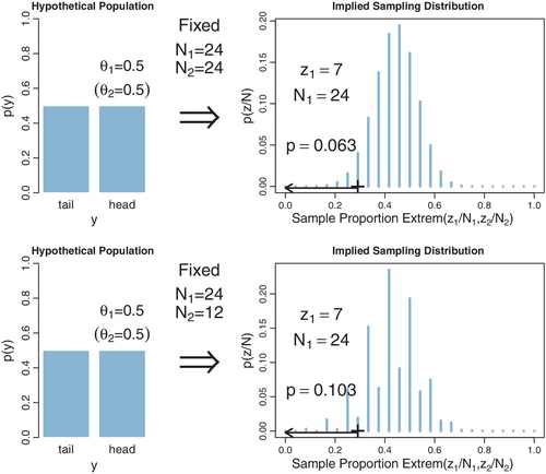
Notice that we do not need to know the result of the second coin (i.e., z₂) to compute the p value of the first coin. In fact, we do not need to flip the second coin at all. All we need for computing the p value for the first coin is the intention to flip the second coin N₂ times. The cloud of imaginary possibilities is determined by sampling intentions, not by observed data.

Figure 11.6 shows another scenario in its lower half, wherein the second coin is flipped only N₂ = 12 times instead of 24 times. With so few flips, it is relatively easy for the second coin to exhibit an extreme outcome by chance alone, even if the null hypothesis is true. Therefore the p value for the first coin gets even larger than before, here up to p = 10.3%, because the space of possible outcomes from both coins now includes many more extreme outcomes.

It might seem artificial to compute a p value for one outcome based on possible results from other outcomes, but this is indeed a crucial concern in NHST. There is a vast literature on “correcting” the p value of one outcome when making multiple tests of other outcomes. As mentioned earlier, typical textbooks in NHST describe at least some of these corrections, usually in the context of analysis of variance (which involves multiple groups of metric data, as we will see in Chapter 19) and rarely in the context of proportions for dichotomous data.⁵

11.1.6 Soul searching

A defender of NHST might argue that I'm quibbling over trivial differences in the p values (although going from p = 1.7% in Figure 11.4 to p = 10.3% in Figure 11.6 is hard to ignore), and, for the examples I've given above, the differences get smaller when N gets larger. There are two flaws in this argument. First, it does not deny the problem, and gives no solution when N is small. Second, it understates the problem because there are many other examples in which the p values differ dramatically across sampling intentions, even for large N. In particular, as we will see in more detail later, when a researcher merely intends to make multiple comparisons across different conditions or parameters, the p value for any single comparison increases greatly.

Defenders of NHST might argue that the examples regarding the stopping intention are irrelevant, because it is okay to compute a p value for every set of data as if N were fixed in advance. The reason it is okay to conditionalize on N (that is, to consider only the observed N column in the z, N outcome space) is that doing so will result in exactly 5% false alarms in the long run when the null hypothesis is true. One expression of this idea comes from Anscombe (1954, p. 91), who stated, “In any experiment or sampling inquiry where the number of observations is an uncertain quantity but does not depend on the observations themselves, it is always legitimate to treat the observations in the statistical analysis as if their number had been fixed in advance. We are then in fact using perfectly correct conditional probability distributions.” The problem with this argument is that it applies equally well to the other stopping rules for computing p values. It is important to notice that Anscombe did not say it is uniquely or only legitimate to treat N as fixed in advance. Indeed, if we treat z as fixed in advance, or if we treat duration as fixed in advance, then we still have perfectly correct conditional probability distributions that result in 5% false alarms in the long run when the null hypothesis is true. The p values for individual data sets may differ, but across many data sets the long-run false alarm rate is 5%. Note also that Anscombe concluded that this whole issue would be avoided if we did Bayesian analysis instead. Anscombe (1954, p. 100) said, “All risk of error is avoided if the method of analysis uses the observations only in the form of their likelihood function, since the likelihood function (given the observations) is independent of the sampling rule. One such method of analysis is provided by the classical theory of rational belief, in which a distribution of posterior probability is deduced, by Bayes’ theorem, from the likelihood function of the observations and a distribution of prior probability.”

Within the context of NHST, the solution is to establish the true intention of the researcher. This is the approach taken explicitly when applying corrections for multiple tests. The analyst determines what the truly intended tests are, and determines whether those testing intentions were honestly conceived a priori or post hoc (i.e., motivated only after seeing the data), and then computes the appropriate p value. The same approach should be taken for stopping rules: The data analyst should determine what the truly intended stopping rule was, and then compute the appropriate p value. Unfortunately, determining the true intentions can be difficult. Therefore, perhaps researchers who use p values to make decisions should be required to publicly pre-register their intended stopping rule and tests, before collecting the data. (There are other motivations for pre-registering research, such as preventing selective inclusion of data or selective reportage of results. In the present context, I am focusing on pre-registration as a way to establish p values.) But what if an unforeseen event interrupts the data collection, or produces a windfall of extra data? What if, after the data have been collected, it becomes clear that there should have been other tests? In these situations, the p values must be adjusted despite the pre-registration. Fundamentally, the intentions should not matter to the interpretation of the data because the propensity of the coin to come up heads does not depend on the intentions of the flipper (except when the stopping rule biases the data collection). Indeed, we carefully design experiments to insulate the coins from the intentions of the experimenter.⁶

11.1.7 Bayesian analysis

The Bayesian interpretation of data does not depend on the covert sampling and testing intentions of the data collector. In general, for data that are independent across trials (and uninfluenced by the sampling intention), the probability of the set of data is simply the product of the probabilities of the individual outcomes. Thus, for $z={\displaystyle {\sum }_{i=1}^N{\gamma }_i}$ heads in N flips, the likelihood is ${\Pi }_{i=1}^N\text{?}{\theta }^{{\gamma }_i}\text{?}{\left(1-\theta \right)}^{1-{\gamma }_i}={\theta }^z\text{?}{\left(1-\theta \right)}^{N-z}$. The likelihood function captures everything we assume to influence the data. In the case of the coin, we assume that the bias (θ) of the coin is the only influence on its outcome, and that the flips are independent. The Bernoulli likelihood function completely captures those assumptions.

In summary, the NHST analysis and conclusion depend on the covert intentions of the experimenter, because those intentions define the probabilities over the space of all possible (unobserved) data, as depicted by the imaginary clouds of possibilities in Figure 11.1, p. 299. This dependence of the analysis on the experimenter's intentions conflicts with the opposite assumption that the experimenter's intentions have no effect on the observed data. The Bayesian analysis, on the other hand, does not depend on the imaginary cloud of possibilities. The Bayesian analysis operates only with the actual data obtained.

11.2.1 NHST analysis

The NHST analysis does not care if we are flipping coins or nails. The analysis proceeds the same way as before. As we saw in the previous sections, if we declare that the intention was to flip the nail 24 times, then an outcome of 7 heads means we do not reject the hypothesis that the nail is fair (recall Figure 11.3, where p > 2.5%). Let me say that again: We have a nail for which we have a strong prior belief that it is tail biased. We flip the nail 24 times, and find it comes up heads 7 times. We conclude, therefore, that we cannot reject the null hypothesis that the nail can come up heads or tails 50/50. Huh? This is a nail we're talking about. How can you not reject the null hypothesis?

11.2.2 Bayesian analysis

The Bayesian statistician starts the analysis with an expression of the prior knowledge. We know from prior experience that the narrow-headed nail is biased to show tails, so we express that knowledge in a prior distribution. In a scientific setting, the prior is established by appealing to publicly accessible and reputable previous research. In our present fictional example involving a nail, suppose that we represent our prior beliefs by a fictitious previous sample that had 95% tails in a sample size of 20. That translates into a beta(θ|2,20) prior distribution if the “proto-prior,” before the fictional data, was beta(θ|1,1). If we wanted to go through the trouble, we could instead derive a prior from established theories regarding the mechanics of such objects, after making physical measurements of the nail such as its length, diameter, mass, rigidity, etc. In any case, to make the analysis convincing to a scientific audience, the prior must be cogent to that audience. Suppose that the agreed prior for the nail is beta(θ|2,20), then the posterior distribution is beta (θ|2 + 7,20 + 17), as shown in the left side of Figure 11.7. The posterior 95% highest density interval (HDI) clearly does not include the nail being fair.

On the other hand, if we have prior knowledge that the object is fair, such as a coin, then the posterior distribution is different. For example, suppose that we represent our prior beliefs by a fictitious previous sample that had 50% tails in a sample size of 20. That translates into a beta(θ|11,11) prior distribution if the “proto-prior,” before the fictional data, was beta(θ|1,1). Then the posterior distribution is beta(θ|11 + 7,11 + 17), as shown in the right side of Figure 11.7. The posterior 95% HDI includes the nail being fair.

The differing inferences for a coin and a nail make good intuitive sense. Our posterior beliefs about the bias of the object should depend on our prior knowledge of the object: 7 heads in 24 flips of narrow-headed nail should leave us with a different opinion than 7 heads in 24 flips of a coin. For additional details and a practical example, see Lindley and Phillips (1976). Despite the emphasis here on the important and appropriate role of prior knowledge, please remember that the prior distributions are overwhelmed with sufficiently large data sets, and the posterior distributions converge to the same result.

11.3.1 CI depends on intention

The primary goal of NHST is determining whether a particular “null” value of a parameter can be rejected. One can also ask what range of parameter values would not be rejected. This range of nonrejectable parameter values is called the CI. (There are different ways of defining an NHST CI; this one is conceptually the most general and coherent with NHST precepts.) The 95% CI consists of all values of θ that would not be rejected by a (two-tailed) significance test that allows 5% false alarms.

For example, in a previous section we found that θ = 0.5 would not be rejected when z = 7 and N = 24, for a data collector who intended to stop when N = 24. The question is, which other values of θ would we not reject? Figure 11.8 shows the sampling distribution for different values of θ. The upper row shows the case of θ = 0.126, for which the sampling distribution has a p value of almost exactly 2.5%. In fact, if θ is nudged any smaller, p becomes smaller than 2.5%, which means that smaller values of θ can be rejected. The lower row of Figure 11.8 shows the case of θ = 0.511, for which the sampling distribution shows p is almost exactly 2.5%. If θ is nudged any larger, then p falls below 2.5%, which means that larger values of θ can be rejected. In summary, the range of θ values we would not reject is θ [0.126,0.511]. This is the 95% confidence interval when z = 7 and N = 24, for a data collector who intended to stop when N = 24. Exercise 11.2 has you examine this “hands-on.”

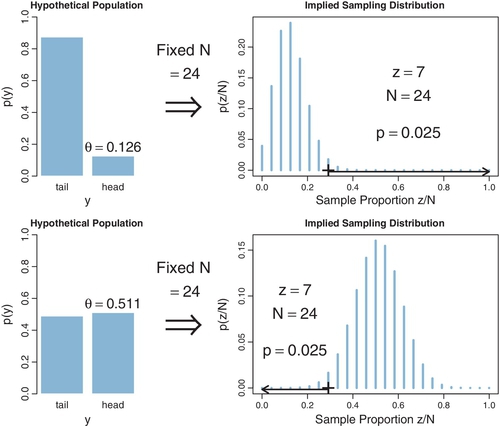
Notice that the CI describes the limits of the θ value, which appear in the left side of Figure 11.8. The parameter θ describes the hypothetical population. Although θ exists on a range from 0 to 1, it is quite different than the sample proportion, z/N, on the right of the figure. Notice also that the sampling distribution is a distribution over the sample proportion; the sampling distribution is not a distribution over the parameter θ. The CI is simply the smallest and largest values of θ that yield p ≥ 2.5%.

We can also determine the CI for the experimenter who intended to stop when z = 7. Figure 11.9 shows the sampling distribution for different values of θ. The upper row shows the case of θ = 0.126, for which the sampling distribution has p = 2.5%. In fact, if θ is nudged any smaller, p is less than 2.5%, which means that smaller values of θ can be rejected. The lower row of Figure 11.9 shows the case of θ = 0.484, for which the sampling distribution has p = 2.5%. If θ is nudged any larger, p falls below 2.5%, which means that larger values of θ can be rejected. In summary, the range of θ values we would not reject is θ [0.126,0.484]. This is the 95% CI when z = 7 and N = 24, for a data collector who intended to stop when z = 7.

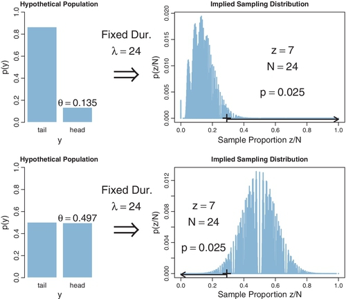
Furthermore, we can determine the CI for the experimenter who intended to stop when a fixed duration expired. Figure 11.10 shows the sampling distribution for different values of θ. The upper row shows the case of θ = 0.135, for which the sampling distribution has p = 2.5%. If θ is nudged any smaller, p is less than 2.5%, which means that smaller values of θ can be rejected. The lower row of Figure 11.9 shows the case of θ = 0.497, for which the sampling distribution has p = 2.5%. If θ is nudged any larger, p falls below 2.5%, which means that larger values of θ can be rejected. In summary, the range of θ values we would not reject is θ [0.135,0.497]. This is the 95% CI when z = 7 and N = 24, for a data collector who intended to stop when time expired.

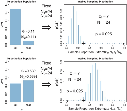
Finally, we can determine the CI for the experimenter who intended to test two coins, with a fixed N for both coins. Figure 11.11 shows the sampling distribution for different values of θ⁷. The upper row shows the case of θ = 0.110, for which the sampling distribution has p = 2.5%. If θ is nudged any smaller, p is less than 2.5%, which means that smaller values of θ can be rejected. The lower row of Figure 11.11 shows the case of θ = 0.539, for which the sampling distribution has p = 2.5%. If θis nudged any larger, p falls below 2.5%, which means that larger values of θ can be rejected. In summary, the range of θ values we would not reject is θ [0.110, 0.539]. This is the 95% CI when z = 7 and N = 24, for a data collector who intended to test two coins and stop when N reached a fixed value.

We have just seen that the NHST CI depends on the stopping and testing intentions of the experimenter. When the intention was to stop when N = 24, then the range of biases that would not be rejected is θ [0.126,0.511]. But when the intention was to stop when z = 7, then the range of biases that would not be rejected is θ [0.126,0.484]. And when the intention was to stop when time was up, then the range of biases that would not be rejected is θ [0.135, 0.497]. And when the intention was to test two coins, stopping each at fixed N, then the CI was θ [0.110, 0.539]. The CI depends on the experimenter's intentions because the intentions determine the cloud of imaginary possibilities relative to which the actually observed data are judged. Thus, the interpretation of the NHST CI is as cloudy as the interpretation of NHST itself, because the CI is merely the significance test conducted at every candidate value of θ. Because CIs are defined by p values, for every misconception of p values, there can be a corresponding misconception of CIs. Although motivated somewhat differently, a similar conclusion was colorfully stated by Abelson (1997, p. 13): “under the Law of Diffusion of Idiocy, every foolish application of significance testing will beget a corresponding foolish practice for confidence limits”

11.3.2 Bayesian HDI

A concept in Bayesian inference, that is somewhat analogous to the NHST CI, is the HDI, which was introduced in Section 4.3.4, p. 87. The 95% HDI consists of those values of θ that have at least some minimal level of posterior credibility, such that the total probability of all such θ values is 95%.

Let's consider the HDI when we flip a coin and observe z = 7 and N = 24. Suppose we have a prior informed by the fact that the coin appears to be authentic, which we express here, for illustrative purposes, as a beta(θ|11,11) distribution. The right side of Figure 11.7 shows that the 95% HDI goes from θ = 0.254 to θ = 0.531. These limits span the 95% most credible values of the bias. Moreover, the posterior density shows exactly how credible each bias is. In particular, we can see that θ = 0.5 is within the 95% HDI. Rules for making discrete decisions are discussed in Chapter 12.

There are at least three advantages of the HDI over an NHST CI. First, the HDI has a direct interpretation in terms of the credibilities of values of θ. The HDI is explicitly about p(θ| D), which is exactly what we want to know. The NHST CI, on the other hand, has no direct relationship with what we want to know; there's no clear relationship between the probability of rejecting the value θ and the credibility of θ. Second, the HDI has no dependence on the sampling and testing intentions of the experimenter, because the likelihood function has no dependence on the sampling and testing intentions of the experimenter.⁸ The NHST confidence interval, in contrast, tells us about probabilities of data relative to imaginary possibilities generated from the experimenter's intentions.

Third, the HDI is responsive to the analyst's prior beliefs, as it should be. The Bayesian analysis indicates how much the new data should alter our beliefs. The prior beliefs are overt and publicly decided. The NHST analysis, on the contrary, does not incorporate prior knowledge.

11.4.1 NHST correction for experiment wise error

When there are multiple groups, it often makes sense to compare each group to every other group. With nine fielding positions, for example, there are 36 different pairwise comparisons we can make. The problem is that each comparison involves a decision with the potential for false alarm, and the p values for all comparisons increase. We already saw, in Section 11.1.5 (p. 310), that the intention to make multiple tests increases the p value because the imaginary cloud of possible outcomes expands. In NHST, we have to take into account all comparisons we intend for the whole experiment. Suppose we set a criterion for rejecting the null such that each decision has a “per-comparison” (PC) false alarm rate of α_PC, e.g., 5%. Our goal is to determine the overall false alarm rate when we conduct several comparisons. To get there, we do a little algebra. First, suppose the null hypothesis is true, which means that the groups are identical, and we get apparent differences in the samples by chance alone. This means that we get a false alarm on a proportion α_PC of replications of a comparison test. Therefore, we do not get a false alarm on the complementary proportion 1 − α_PC of replications. If we run c independent comparison tests, then the probability of not getting a false alarm on any of the tests is (1 − α_PC)^c. Consequently, the probability of getting at least one false alarm is 1 − (1 − α_PC)^c. We call that probability of getting at least one false alarm, across all the comparisons in the experiment, the “experimentwise” false alarm rate, denoted α_EW. Here's the rub: α_EW is greater than α_PC. For example, if α_PC = .05 and c = 36, then α_EW = 1 − (1 − α_PC)^c = 0.84. Thus, even when the null hypothesis is true, and there are really no differences between groups, if we conduct 36 independent comparisons, we have an 84% chance of falsely rejecting the null hypothesis for at least one of the comparisons. Usually not all comparisons are structurally independent of each other, so the false alarm rate does not increase so rapidly, but it does increase whenever additional comparison tests are conducted.

One way to keep the experimentwise false alarm rate down to 5% is by reducing the permitted false alarm rate for the individual comparisons, i.e., setting a more stringent criterion for rejecting the null hypothesis in individual comparisons. One often-used resetting is the Bonferonni correction,which sets ${\alpha }_{\text{PC}}={\alpha }_{\text{EW}}^{\text{desired}}/c$. For example, if the desired experimentwise false alarm rate is 0.05, and there are 36 comparisons planned, then we set each individual comparison's false alarm rate to 0.05/36. This is a conservative correction, because the actual experimentwise false alarm rate will usually be much less than ${\alpha }_{\text{EW}}^{\text{desired}}$.

There are many different corrections available to the discerning NHST aficionado (e.g., Maxwell & Delaney, 2004, chap. 5). Not only do the correction factors depend on the structural relationships of the comparisons, but the correction factors also depend on whether the analyst intended to conduct the comparison before seeing the data, or was provoked into conducting the comparison only after seeing the data. If the comparison was intended in advance, it is called a planned comparison. If the comparison was thought of only after seeing a trend in the data, it is called a post hoc comparison. Why should it matter whether a comparison is planned or post hoc? Because even when the null hypothesis is true, and there are no real differences between groups, there will always be a highest and lowest random sample among the groups. If we don't plan in advance which groups to compare, but do compare whichever two groups happen to be farthest apart, we have an inflated chance of declaring groups to be different that aren't truly different.

The point, for our purposes, is not which correction to use. The point is that the NHST analyst must make some correction, and the correction depends on the number and type of comparisons that the analyst intends to make. This creates a problem because two analysts can come to the same data but leave with different conclusions because of the variety of comparisons that they find interesting enough to conduct, and what provoked their interest. The creative and inquisitive analyst, who wants to conduct many comparisons either because of deep thinking about implications of theory, or because of provocative unexpected trends in the data, is penalized for being thoughtful. A large set of comparisons can be conducted only at the cost of using a more stringent threshold for each comparison. The uninquisitive analyst is rewarded with an easier criterion for achieving significance. This seems to be a counterproductive incentive structure: You have a higher chance of getting a “significant” result, and getting your work published, if you feign narrow mindedness under the pretense of protecting the world from false alarms.

To make this concrete, consider again the estimation of baseball batting abilities for players from different fielding positions, in Section 9.5.1 (p. 253). A basic question might be whether the batting ability of infielders differs from the batting ability of outfielders. Therefore an uninquisitive analyst might plan to make the single comparison of the average of the six non-outfield positions against the average of the three outfield positions. A more inquisitive or knowledgeable analyst might plan additional comparisons, suspecting that pitchers and catchers might be different from basemen because of the different skills demanded for the pitcher-catcher duo. This analyst might plan four comparisons: outfielders versus non-outfielders, outfielders versus basemen, outfielders versus average of catchers and pitchers, and basemen versus average of catchers and pitchers. The more inquisitive and knowledgeable analyst is punished with a more stringent criterion for declaring significance, even on the comparison of outfielders versus non-outfielders that the uninquisitive analyst also made.

Suppose that, upon seeing the data, the detail-oriented analyst discovers that catchers actually have about the same batting average as basemen, and therefore comparison should be made between catchers and basemen and between catchers and pitchers. The analyst should treat this as a post hoc, not planned, comparison. But wait—upon reflection, it is clear merely from knowledge of the game that catchers have much different demands than pitchers, and therefore these comparisons should have been considered from the start. So, perhaps these comparisons should be considered planned, not post hoc, after all. Suppose also that, upon seeing the data, the analyst notices that the basemen don't differ much from the outfielders. Therefore it seems superfluous to compare them. This lack of comparison is post hoc, because a comparison had been planned. But, in retrospect, it's clear from background knowledge about the game that basemen and outfielders actually have similar demands: they all must catch fly balls and throw to basemen. Therefore the lack of comparison should have been planned after all.

All this leaves the NHST analyst walking on the quicksand of soul searching. Was the comparison truly planned or post hoc? Did the analyst commit premeditated exclusion of comparisons that should have been planned, or was the analyst merely superficial, or was the exclusion post hoc? This problem is not solved by picking a story and sticking to it, because any story still presumes that the analyst's testing intentions should influence the data interpretation.

11.4.2 Just one Bayesian posterior no matter how you look at it

The data from an experiment, or from an observational study, are carefully collected so to be totally insulated from the experimenter's intentions regarding subsequent tests. In experiments, each datum should be uninfluenced by the presence or absence of any other condition or subject in the experiment. For properly conducted experiments, in which subjects are kept uninformed about the goals or structure of the experiment (until after the experiment is done), there is no way for an individual in one experimental group to be influenced by the presence or absence of any groups or subjects, before or after. Moreover, the data are uninfluenced by the experimenter's intentions regarding the other groups and sample size.

In a Bayesian analysis, the interpretation of the data is not influenced by the experimenter's stopping and testing intentions (assuming that those intentions do not affect the data). A Bayesian analysis yields a posterior distribution over the parameters of the model. The posterior distribution is the complete implication of the data. The posterior distribution can be examined in as many different ways as the analyst deems interesting; various comparisons of groups are merely different perspectives on the posterior distribution.

For example, in the baseball data we examined several comparisons of different positions (e.g., Figure 9.14) and of different individual players (e.g., Figure 9.15). Those marginal distributions merely summarize the posterior distribution from various perspectives. The posterior distribution itself is unchanged by how we look at it. We can examine any other comparison of parameters without worrying about what motivated us to consider it, because the posterior distribution is unchanged by those motivations, unlike the cloud of imaginary possibilities from the null hypothesis.

In summary, the Bayesian posterior distribution is appropriately insensitive to the experimenter's stopping and sampling intentions to compare or not compare various groups. The Bayesian posterior also directly tells us the credibilities of the magnitudes of differences, unlike NHST which tells us only about whether a difference is extreme in a cloud of possibilities determined by the experimenter's intentions.

11.4.3 How Bayesian analysis mitigates false alarms

No analysis is immune to false alarms, because randomly sampled data will occasionally contain accidental coincidences of outlying values. Bayesian analysis eschews the use of p values as a criterion for decision making, however, because p values control false alarms on the basis of the analyst's intentions, not on the basis of the data. Bayesian analysis instead accepts the fact that the posterior distribution is the best inference we can make, given the observed data and the prior knowledge.

How, then, does a Bayesian analysis address the problem of false alarms? By incorporating prior knowledge into the structure of the model. Specifically, if we know that different groups have some overarching commonality, even if their specific treatments are different, we can nevertheless describe the different group parameters as having been drawn from an overarching distribution that expresses the commonality. Examples of hierarchical models were given in Figures 9.7 (p. 236, re therapeutic touch) and 9.13 (p. 252, re baseball batting ability). If several of the groups yield similar data, this similarity informs the overarching distribution, which in turn implies that any outlying groups should be estimated to be a little more similar than they would be otherwise. In other words, just as there can be shrinkage of individual estimates toward the group central tendency, there can be shrinkage of group estimates toward the overall central tendency. Shrinkage was described extensively in Section 9.3 (p. 245). The shrinkage pulls in the estimates of accidental outliers and reduces false alarms (e.g., D. A. Berry & Hochberg, 1999; Gelman, 2005; Gelman, Hill, & Yajima, 2009; Lindquist & Gelman, 2009; Meng & Dempster, 1987). This shrinkage is not an arbitrary “correction” like those applied in NHST. The shrinkage is a rational consequence of the prior knowledge expressed in the model structure. Hierarchical structure can be put into models that are assessed using NHST, but Bayesian estimation is especially seamless and straightforward for implementing and evaluating hierarchical models.

11.5.1 Planning an experiment

So far in this book, we have only considered the analysis of data that have already been obtained. But a crucial part of conducting research is planning the study before actually obtaining the data. When planning research, we have some hypothesis about how the world might be, and we want to gather data that will inform us about the viability of that hypothesis. Typically we have some notion already about the experimental treatments or observational settings, and we want to plan how many observations we'll probably need to make, or how long we'll need to run the study, in order to have reasonably reliable evidence one way or the other.

For example, suppose that my theory suggests a coin should be biased with θ around 0.60, perhaps a little higher and perhaps a little lower. The coin might represent a population of voters, hence flipping the coin means polling a person in the population, and the outcome heads means preference for candidate A. The theory regarding the bias may have come from previous polls regarding political attitudes. We would like to plan a survey of the population that will give us precise posterior beliefs about the true preference for candidate A. Suppose we contemplate a survey that polls 500 people. By simulating the experiment over and over, using the hypothesized random θ ≈ 0.60 and N = 500, we can generate simulated data, and then derive a Bayesian posterior distribution for every set of simulated data. For every posterior distribution, we determine some measure of accuracy, such as the width of the 95% HDI. From many simulated experiments, we get a sampling distribution of HDI widths. From the sampling distribution of HDI widths, we can decide whether N = 500 typically yields high enough accuracy for our purposes. If not, we repeat the simulation with a larger N. Once we know how big N needs to be to get the accuracy we seek, we can decide whether or not it is feasible to conduct such a study.

Notice that we used the intended experiment to generate a space of possible data in order to anticipate what is likely to happen when the data are analyzed with Bayesian methods. For any single set of data (simulated or actual), we recognize that the individual data points in the set are insulated from the intentions of the design, and we conduct a Bayesian analysis of the data set. The use of a distribution of possible sample data, from an intended experiment, is perfectly appropriate here because it is exactly the implications of this hypothetical data distribution that we want to discover.

The issues of research design will be explored in depth in Chapter 13. You might want to glance at Figure 13.1, p. 363, to see how a cloud of possible data is used as a “dress rehearsal” for planning actual data collection. In particular, notice that a Bayesian analysis of actual data, illustrated in the top panel of Figure 13.1, does not use a cloud of possibilities from a hypothesis, and is quite different from the construction of p values illustrated in Figure 11.1, p. 299.

11.5.2 Exploring model predictions (posterior predictive check)

A Bayesian analysis only indicates the relative credibilities of the various parameter values or models under consideration. The posterior distribution only tells us which parameter values are relatively less bad than the others. The posterior does not tell us whether the least bad parameter values are actually any good.

For example, suppose we believe that a coin is a heavily biased trick coin, and either comes up heads 99% of the time, or else comes up tails 99% of the time; we just don't know which direction of bias it has. Now we flip the coin 40 times and it comes up heads 30 of those flips. It turns out that the 99%-head model has a far bigger posterior probability than the 99%-tail model. But it is also the case that the 99%-head model is a terrible model of a coin that comes up heads 30 out of 40 flips!

One way to evaluate whether the least unbelievable parameter values are any good is via a posterior predictive check. A posterior predictive check is an inspection of patterns in simulated data that are generated by typical posterior parameters values. The idea of a posterior predictive check is as follows: If the posterior parameter values really are good descriptions of the data, then the predicted data from the model should actually “look like” real data. If the patterns in the predicted data do not mirror the patterns in the actual data, then we are motivated to invent models that can produce the patterns of interest.

This use of the posterior predictive check is suspiciously like NHST: We start with a hypothesis (i.e., the least unbelievable parameter values), and we generate simulated data as if we were repeating our intended experiment over and over. Then we see if the actual data are typical or atypical in the space of simulated data. If we were to go further, and determine critical values for false alarm rates and then reject the model if the actual data fall in its extreme tails, then we would indeed be doing something tantamount to NHST. Some authors do promote this sort of “Bayesian p value.” But I prefer to keep posterior predictive checks fully Bayesian. The goal of the posterior predictive check is to drive intuitions about the qualitative manner in which the model succeeds or fails, and about what sort of novel model formulation might better capture the trends in the data. Once we invent another model, then we can use Bayesian methods to quantitatively compare it with the other models. For further discussion, see Section 17.5.1 andKruschke (2013b).