
Nominal Predicted Variable
Just when dichotomous, metric, were sure,
Multiple nominal outcomes occur.
Just when you thought you might rest and relax,
Here come logistics of linking softmax.1
This chapter considers data structures that have a nominal predicted variable. When the nominal predicted variable has only two possible values, this reduces to the case of the dichotomous predicted variable considered in the previous chapter. In the present chapter, we generalize to cases in which the predicted variable has three or more categorical values. For example, we might want to predict a person's political party affiliation (a nominal variable) based on their annual income and years of education. Or we might want to predict the species of fish (a nominal variable) we are likely to observe based on the salinity and temperature of the water.
The traditional treatment of this sort of data structure is called multinomial logistic regression or conditional logistic regression. We will consider Bayesian approaches to these methods. As usual, in Bayesian software it is easy to generalize the traditional models so they are robust to outliers, allow different variances within levels of a nominal predictor, and have hierarchical structure to share information across levels or factors as appropriate.
In the context of the generalized linear model (GLM) introduced in Chapter 15, this chapter's situation involves a link function that is the so-called softmax along with a categorical distribution for describing noise in the data, as indicated in the third row of Table 15.2 (p. 443). For a reminder of how this chapter's combination of predicted and predictor variables relates to other combinations, see Table 15.3 (p. 444).
22.1 Softmax regression
The usual generalizations of logistic regression are of two types: conditional logistic regression, which will be explored later in the chapter, and so-called multinomial logistic regression, which we explore in this section. I am not fond of the traditional name, however, because the model does not use the logistic function per se, so the name “logistic” is a misnomer, and all the models in this chapter describe multinomial data, so the name “multinomial” is not informative. Instead, the key descriptor of the model is its inverse-link function, which is the softmax function (which will be defined below). Therefore, I refer to the method as softmax regression instead of multinomial logistic regression.
In the previous chapter, we used the logistic function to go from a linear combination of predictors to the probability of outcome 1 relative to outcome 0. In this chapter, we want to generalize to multiple categorical outcomes. The generalization of the logistic function requires a bit of mathematical development, but it's really just repeated algebraic manipulation of exponential functions, so don't be deterred. To keep the notation reasonably simple, we will suppose that we have a single metric predictor, x. All the derivations below easily generalize to multiple predictors. The underlying linear propensity of outcome k is denoted
The subscripts k indicate that there is an equation like Equation 22.1 for every outcome category. We call the set of possible outcomes S. Now a novelty: The probability of outcome k is given by the softmax function:
In words, Equation 22.2 says that the probability of outcome k is the exponentiated linear propensity of outcome k relative to the sum of exponentiated linear propensities across all outcomes in the set S. You may be wondering, Why exponentiate? Intuitively, we have to go from propensities that can have negative values to probabilities that can only have non-negative values, and we have to preserve order. The exponential function satisfies that need.
The softmax function is used in many applications as a way of mapping several real-valued variables to order-preserving outcome probabilities (e.g., Bishop, 2006). It is called the softmax function because when it is given another parameter, called the gain γ, that amplifies all the inputs, then the softmax assigns the maximum input with nearly 100% probability when the gain is large:
The softmax formulation can be useful for applications that use the derivative (i.e., gradient) to find optimal input values, because gradient ascent requires smooth differentiable functions (cf., Kruschke & Movellan, 1991).
It turns out that there are indeterminacies in the system of Equations 22.1 and 22.2. We can add a constant C0 to every β0,k, and add a constant C1 to every β1, k, and get exactly the same probabilities of responding with each category:

Therefore, we can set the baseline and slope for one of the response categories to arbitrary convenient constants. We will set the constants of one response category, called the reference category r, to zero: β0, r =0 and β1, r =0.
Because of the indeterminacy in the regression coefficients, we can interpret the regression coefficients only relative to the reference category. ![]() ecall from Section 21.2.1 (p. 629) that the regression coefficients in logistic regression can be conceived in terms of log odds of outcome 1 relative to outcome 0. In the present application, the regression coefficients can be conceived in terms of the log odds of each outcome relative to the reference outcome:
ecall from Section 21.2.1 (p. 629) that the regression coefficients in logistic regression can be conceived in terms of log odds of outcome 1 relative to outcome 0. In the present application, the regression coefficients can be conceived in terms of the log odds of each outcome relative to the reference outcome:

In other words, the regression coefficient β1, k is the increase in log odds of outcome k relative to the reference outcome r for a one-unit increase in x.
Figure 22.1 shows two examples of data generated from the multinomial logistic model. The examples use two predictors (x1 and x2) to better illustrate the variety of patterns that can be produced by the model. The regression coefficients are displayed in the titles of the panels within the figure. The regression coefficients are large on the scale of x so that the transitions across outcomes are visually crisp. In realistic data, the regression coefficients are usually of much smaller magnitude and the outcomes of all types extensively overlap.
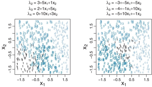
For the examples in Figure 22.1, the reference outcome was chosen to be 1, so all the regression coefficients describe the log odds of the other outcomes relative to outcome 1. Consider outcome 2, which has log odds specified by the regression coefficients for λ2. If, for λ2, the regression coefficient on x1 is positive, then the probability of outcome 2, relative to outcome 1, goes up as x1 increases. And, still for λ2, if the regression coefficient on x2 is positive, then the probability of outcome 2, relative to outcome 1, goes up as x2 increases. The baseline, β0 determines how large x1 and x2 need to become for the probability of outcome 2 to exceed the probability of outcome 1: The larger the baseline, the smaller x1 and x2 need to be.
You can see these trends occur in the two panels of Figure 22.1. In each panel, locate the region in which the reference outcome (i.e., 1) occurs. If λ2's coefficient on x1 is positive, then the region in which outcome 2 occurs will tend to be on the right of the region where the reference outcome occurs. If λ2's coefficient on x1 is negative, then the region in which outcome 2 occurs will tend to be on the left of the region where the reference outcome occurs. Analogously for x2: If λ2's coefficient on x2 is positive, then the region in which outcome 2 occurs will tend to be above the region where the reference outcome occurs. If λ2's coefficient on x2 is negative, then the region in which outcome 2 occurs will tend to be below the region where the reference outcome occurs. These trends apply to the other outcomes as well.
Another general conclusion to take away from Figure 22.1 is that the regions of the different outcomes do not necessarily have piecewise linear boundaries. Later in the chapter we will consider a different sort of model that always produces outcome regions that have piecewise linear boundaries.
22.1.1 Softmax reduces to logistic for two outcomes
When there are only two outcomes, the softmax formulation reduces to the logistic regression of Chapter 21. The reference outcome is declared to be outcome y = 0, and the regression coefficients describe the log odds of outcome y = 1 relative to outcome y = 0. To make this explicit, let's see how the softmax function of exponentiated linear propensities becomes the logistic function when there are just two outcome categories. We start with the definition of the softmax function in Equation 22.2 and algebraically re-arrange it for the case of two outcome categories:

Thus, softmax regression is one natural generalization of logistic regression. We will see a different generalization later in the chapter.
22.1.2 Independence from irrelevant attributes
An important property of the softmax function of Equation 22.2 is known as independence from irrelevant attributes (Luce, 1959, 2008). The model implies that the ratio of probabilities of two outcomes is the same regardless of what other possible outcomes are included in the set. Let S denote the set of possible outcomes. Then, from the definition of the softmax function, the ratio of outcomes j and k is

The summation in the denominators cancels and has no effect on the ratio of probabilities. Obviously if we changed the set of outcomes S to any other set S* that still contains outcomes j and k, the summation Σc ∈ S* would still cancel and have no effect on the ratio of probabilities.
An intuitive example that obeys independence from irrelevant attributes is as follows. Suppose there are three ways to get from home to work, namely walking, bicycling, or bussing. Suppose that a person prefers walking the best, followed by bicycling, followed by bussing, and suppose that choosing a method is probabilistic with ratios of 3:2:1, which is to say that walking is chosen 3 to 2 over bicycling, which is chosen 2 to 1 over bussing. In other words, there is a 50% chance of walking, a 33.3% chance of bicycling, and a 16.7% chance of bussing. The ratio of the probability of walking to the probability of bussing is 3:1. Now, suppose one day the bicycle has a flat tire, so the outcome set is reduced. It makes intuitive sense that there should be the same ratio of probabilities among the remaining options, which is to say that walking should still be preferred to bussing in the ratio 3:1.
But not all situations will be accurately described by independence from irrelevant attributes. Debreu (1960) pointed out an example that violates independence from irrelevant attributes. Suppose there are three ways to get from home to work, namely walking, taking the red bus, or taking the blue bus. Suppose that a person prefers walking to bussing in the ratio 3:1, but is indifferent about red or blue buses. When all three options are available, there is a 75% probability of walking and a 25% probability of taking a bus, which means a 12.5% probability of taking a red bus and a 12.5% probability of taking a blue bus. The ratio of walking to taking a red bus is therefore 6:1. Now, suppose one day the blue bus company breaks down, so the outcome set is reduced. It makes intuitive sense that there should still be a 75% preference for walking and a 25% preference for taking a bus, but now the ratio of walking to taking a red bus is 3:1, not 6:1.
Thus, when applying the descriptive model of Equation 22.2, we are implicitly assuming independence from irrelevant attributes. This might or might not be a reasonable assumption in any given application.
22.2 Conditional logistic regression
Softmax regression conceives of each outcome as an independent change in log odds from the reference outcome, and a special case of that is dichotomous logistic regression. But we can generalize logistic regression another way, which may better capture some patterns of data. The idea of this generalization is that we divide the set of outcomes into a hierarchy of two-set divisions, and use a logistic to describe the probability of each branch of the two-set divisions. The underlying propensity to respond with any outcome in the subset of outcomes S* relative to (i.e., conditional on) a larger set S is denoted
and the conditional response probability is
The thrust of Equations 22.7 and 22.8 is that the regression coefficients refer to the conditional probability of outcomes for the designated subsets, not necessarily to a single outcome among the full set of outcomes.
Figure 22.2 shows two examples of hierarchies of binary divisions of four outcomes. In each example, the full set of (four) outcomes appears at the top of the hierarchy, and the binary divisions progress downward. Each branch is labeled with its conditional probability. For example, the top left branch indicates the occurrence of outcome 1 given the full set, and the conditional probability of this occurrence is labeled ϕ{1}|{1,2,3,4}. This conditional probability will be modeled by a logistic function of the predictors. We will now explore detailed numerical examples of the two hierarchies.

In the left hierarchy of Figure 22.2, we opt to split the outcomes into a hierarchy of binary divisions as follows:
• 2 versus 3 or 4
• 3 versus 4
At each level in the hierarchy, the conditional probability of the options is described by a logistic function of a linear combination of the predictors. For our example, we assume there are two metric predictors. The linear combinations of predictors are denoted

and the conditional probabilities of the outcome sets are simply the logistic function applied to each of the λ values:
The ϕ values, above, should be thought of as conditional probabilities, as marked on the arrows in Figure 22.2. For example, ϕ{2}|{2,3,4} is the probability of outcome 2 given that outcomes 2, 3, or 4 occurred. And the complement of that probability, 1 – ϕ{2}|{2,3,4} is the probability of outcomes 3 or 4 given that outcomes 2, 3, or 4 occurred.
Finally, the most important equations that actually determine the relations between the expressions above, are the equations that specify the probabilities of the individual outcomes as the appropriate combinations of the conditional probabilities. These probabilities of the individual outcomes are determined simply by multiplying the conditional probabilities on the branches of the hierarchy in Figure 22.2 that lead to the individual outcomes. Thus,

Notice that the sum of the outcome probabilities is indeed 1 as it should be; that is, ϕ1 + ϕ2 + ϕ3 + ϕ4 = 1. This result is easiest to verify in this case by summing in the order ((ϕ4+ϕ3)+ϕ2)+ϕ1.
The left panel of Figure 22.3 shows an example of data generated from the conditional logistic model of Equations 22.9–22.11. The x1 and x2 values were randomly generated from uniform distributions. The regression coefficients are displayed in the title of the panel within the figure. The regression coefficients are large compared to the scale of x so that the transitions across outcomes are visually crisp. In realistic data, the regression coefficients are usually of much smaller magnitude and outcomes of all types extensively overlap. You can see in the left panel of Figure 22.3 that there is a linear separation between the region of 1 outcomes and the region of 2, 3, or 4 outcomes. Then, within the region of 2, 3, or 4 outcomes, there is a linear separation between the region of 2 outcomes and the region of 3 or 4 outcomes. Finally, within the region of 3 or 4 outcomes, there is a linear separation between the 3's and 4's. Of course, there is probabilistic noise around the linear separations; the underlying linear separations are plotted where the logistic probability is 50%.

We now consider another example of conditional logistic regression, again involving four outcomes and two predictors, but with a different parsing of the outcomes. The hierarchy of binary partitions of the outcomes is illustrated in the right side of Figure 22.2. In this case, we opt to split the outcomes into the following hierarchy of binary choices:
• 1 versus 2
• 3 versus 4
At each level in the hierarchy, the conditional probability of the options is described by a logistic function of a linear combination of the predictors. For the choices above, the linear combinations of predictors are denoted

and the conditional probabilities of the outcome sets are simply the logistic function applied to each of the λ values:

Finally, the most important equations, that actually determine the relations between the expressions above, are the equations that specify the probabilities of the individual outcomes as the appropriate combinations of the conditional probabilities, which can be gleaned from the conditional probabilities on the branches of the hierarchy in the right side of Figure 22.2. Thus:

Notice that the sum of the outcome probabilities is indeed 1 as it should be; that is, ϕ1 + ϕ2 + ϕ3 + ϕ4 = 1. This result is easiest to verify in this case by summing in the order (ϕ1 + ϕ2) + (ϕ3 + ϕ4). The only structural difference between this example and the previous example is the difference between the forms of Equations 22.11 and 22.14. Aside from that, both examples involve coefficients on predictors where the meaning of the coefficients is determined by how their values are combined in Equations 22.11 and 22.14. The coefficients were given mnemonic subscripts in anticipation of the particular combinations Equations 22.11 and 22.14.
The right panel of Figure 22.3 shows an example of data generated from the conditional logistic model of Equations 22.11–22.14. The regression coefficients are displayed in the title of the panel within the figure. You can see in the right panel of Figure 22.3 that there is a linear separation between the region of 1 or 2 outcomes and the region of 3 or 4 outcomes. Then, within the region of 1 or 2 outcomes, there is a linear separation between the region of 1 outcomes and the region of 2 outcomes. Finally, within the region of 3 or 4 outcomes, there is a linear separation between the 3's and 4's. Of course, there is probabilistic noise around the linear separations; the linear separations are plotted as dashed lines where the logistic probability is 50%.
In general, conditional logistic regression requires that there is a linear division between two subsets of the outcomes, and then within each of those subsets there is a linear division of smaller subsets, and so on. This sort of linear division is not required of the softmax regression model, examples of which we saw in Figure 22.1. You can see that the outcome regions of the softmax regression in Figure 22.1 do not appear to have the hierarchical linear divisions required of conditional logistic regression. ![]() eal data can be extremely noisy, and there can be multiple predictors, so it can be challenging or impossible to visually ascertain which sort of model is most appropriate. The choice of model is driven primarily by theoretical meaningfulness.
eal data can be extremely noisy, and there can be multiple predictors, so it can be challenging or impossible to visually ascertain which sort of model is most appropriate. The choice of model is driven primarily by theoretical meaningfulness.
22.3 Implementation in jags
22.3.1 Softmax model
Figure 22.4 shows a hierarchical diagram for softmax regression. It is directly analogous to the hierarchical diagram for logistic regression, shown here again for convenience (repeated from Figure 21.2, p. 624). The juxtaposition of the diagrams presents another perspective on the fact that logistic regression is a special case of softmax regression.

There are only a few novelties in the diagram for softmax regression in Figure 22.4. Most obviously, at the bottom of the diagram is a distribution named “categorical.” It is just like the Bernoulli distribution but with several outcomes instead of only two. The outcomes are typically named as consecutive integers starting at 1, but this naming scheme does not connote ordering or distance between values. Thus, yi at the bottom of the diagram indicates an integer outcome label for the ith data point. Outcome k has probability denoted μ[k], and the outcome probabilities are visually suggested by the heights of the bars in the icon for the categorical distribution, just as the outcomes of the Bernoulli distribution have probabilities indicated by the heights of its two bars. Moving up the diagram, each outcome's probability is given by the softmax function. The subscript [k] in the softmax function merely suggests that the function is applied to every outcome k.
The model is expressed in JAGS much like logistic regression on metric predictors. The predictor values are standardized to make MCMC sampling more efficient, and the parameters are transformed to the original scale, just as in logistic regression. A novelty comes in computing the softmax function, because JAGS does not have softmax built in (but Stan does). The JAGS code uses a for loop to go through the outcomes and compute the exponentiated λk values from Equation 22.1. The variable explambda [k,i] is the exponentiated λk for the ith data point. Those values are then normalized and used as the probabilities in the categorical distribution, which is denoted in JAGS as dcat. In the JAGS code below, Nout is the number of outcome categories, Nx is the number of predictors, and Ntotal is the number data points. Please read the code below and see if you can make sense of each line. As usual, the lines of JAGS code start at the bottom of the dependency diagram.
The dcat distribution in JAGS automatically normalizes its argument vector, so we do not need to prenormalize its argument. Thus, the explicit normalizing we did above, like this:
could instead be simplified and stated like this:
The simplified form is used in the program Jags-Ynom-XmetMulti-Msoftniax.R, which is called from the high-level script Jags-Ynom-XmetMulti-Msoftmax-Example.R.
22.3.2 Conditional logistic model
The conditional logistic model has all its primary “action” in the outcome-partition hierarchies of Figure 22.2. You can imagine combining an outcome-partition hierarchy of Figure 22.2 with the logistic regression diagram on the right side of Figure 22.4 to create a diagram of a conditional logistic model. Each ϕS*|S in the outcome-partition hierarchy would have its own logistic function. Note that every different outcome-partition hierarchy yields a different conditional logistic model.
Although making a diagram of the model might be challenging, implementing it in JAGS is easy. Consider the outcome-partition hierarchy on the left side of Figure 22.2, with corresponding formal expression in Equations 22.9–22.11. The outcome probabilities, ϕk,for the ith data point are coded in JAGS as mu[k,i]. Take a look at the JAGS code, below, to see the direct implementation of Equations 22.9–22.11. ![]() emember that the logistic function in JAGS is ilogit.
emember that the logistic function in JAGS is ilogit.
The outcome-partition hierarchy on the right-hand side of Figure 22.2, with corresponding formal expression in Equations 22.12–22.14, is virtually identical. The only difference is the specification of the outcome probabilities:
The models are defined in the files named Jags-Ynom-XmetMulti-McondLogistic1.R and Jags-Ynom-XmetMulti-McondLogistic2.R, and are called from the high-level scripts named Jags-Ynom-XmetMulti-McondLogistic1-Example.R and Jags-Ynom-XmetMulti-McondLogistic2-Example.R.
22.3.3 Results: Interpreting the regression coefficients
22.3.3.1 Softmax model
We start by applying the softmax model to some data generated by a softmax model. Figure 22.5 shows the results. The data are reproduced in the left of the figure, and the posterior distribution is shown on the right. The data graph includes, in its title, the values of the regression coefficients that actually generated the data. The estimated parameter values should be near the generating values, but not exactly the same because the data are merely a finite random sample. Each row of marginal posterior distributions corresponds to an outcome value. The top row corresponds to the reference outcome 1, which has regression coefficients set to zero, and the posterior distributions show spikes at zero that confirm this choice of reference outcome. The second row corresponds to outcome 2. Its true regression coefficients are shown in the equation for λ2 above the data graph. You can see that the estimated values are close to the true values. This correspondence of true and estimated parameter values obtains for all the outcome values.

For real data, we usually do not know what process truly generated the data, much less its true parameter values. All we have is a smattering of very noisy data and a posterior distribution on the parameter values of the model that we chose to describe the data. Interpreting the parameters is always contextualized relative to the model. For the softmax model, the regression coefficient for outcome k on predictor xj indicates that rate at which the log odds of that outcome increase relative to the reference outcome for a one unit increase in xj, assuming that a softmax model is a reasonable description of the data.
It is easy to transform the estimated parameter values to a different reference category. ![]() ecall from Equation 22.3 (p. 651) that arbitrary constants can be added to all the regression coefficients without changing the model prediction. Therefore, to change the parameters estimates so they are relative to outcome
ecall from Equation 22.3 (p. 651) that arbitrary constants can be added to all the regression coefficients without changing the model prediction. Therefore, to change the parameters estimates so they are relative to outcome ![]() , we simply subtract
, we simply subtract ![]() from βj,k for all predictors j and all outcomes k. We do this at every step in the MCMC chain. For example, in Figure 22.5, consider the regression coefficient on x1 for outcome 2.
from βj,k for all predictors j and all outcomes k. We do this at every step in the MCMC chain. For example, in Figure 22.5, consider the regression coefficient on x1 for outcome 2. ![]() elative to reference outcome 1, this coefficient is positive, meaning that the probability of outcome 2 increases relative to outcome 1 when x1 increases. You can see this in the data graph, as the region of 2's falls to right side (positive x1 direction) of the region of 1's. But if the reference outcome is changed to outcome 4, then the coefficient on x1 for outcome 2 changes to a negative value. Algebraically this happens because the coefficient on x1 for outcome 4 is larger than for outcome 2, so when the coefficient for outcome 4 is subtracted, the result is a negative value for the coefficient on outcome 2. Visually, you can see this in the data graph, as the region of 2's falls to the left side (negative x1 direction) of the region of 4's. Thus, interpreting regression coefficients in a softmax model is rather different than in linear regression. In linear regression, a positive regression coefficient implies that y increases when the predictor increases. But not in softmax regression, where a positive regression coefficient is only positive with respect to a particular reference outcome.
elative to reference outcome 1, this coefficient is positive, meaning that the probability of outcome 2 increases relative to outcome 1 when x1 increases. You can see this in the data graph, as the region of 2's falls to right side (positive x1 direction) of the region of 1's. But if the reference outcome is changed to outcome 4, then the coefficient on x1 for outcome 2 changes to a negative value. Algebraically this happens because the coefficient on x1 for outcome 4 is larger than for outcome 2, so when the coefficient for outcome 4 is subtracted, the result is a negative value for the coefficient on outcome 2. Visually, you can see this in the data graph, as the region of 2's falls to the left side (negative x1 direction) of the region of 4's. Thus, interpreting regression coefficients in a softmax model is rather different than in linear regression. In linear regression, a positive regression coefficient implies that y increases when the predictor increases. But not in softmax regression, where a positive regression coefficient is only positive with respect to a particular reference outcome.
22.3.3.2 Conditional logistic model
We now apply the conditional logistic models to the data generated by those models. The upper halves of Figures 22.6 and 22.7 show the data and the posterior distributions of the parameters. (The lower halves of the figures will be discussed later.) Superimposed on the data are a smattering of credible 50% threshold lines for each of the conditional logistic functions. You can see that the true parameter values a recovered reasonably well.
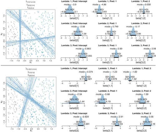

In the upper half of Figure 22.6, consider the estimates of regression coefficients for “Lambda 1.” This corresponds to λ{1}|{1,2,3,4}, which indicates the probability of outcome 1 versus all other outcomes. The estimated coefficient on x1 is negative, indicating that the probability of outcome 1 increases as x1 decreases. The estimated coefficient on x2 is essentially zero, indicating that the probability of outcome 1 is unaffected by changes in x2. This interpretation can also be seen in the threshold lines superimposed on data: The lines separating 1's from other outcomes are essentially vertical. Now consider the regression coefficients for “Lambda 2,” which corresponds to λ{2}|{2,3,4} and indicates the probability of outcome 2 within the zone where outcome 1 does not occur. The estimated coefficient on x2 is negative, which means that the probability of outcome 2 increases as x2 decreases, again within the zone where outcome 1 does not occur. In general, regression coefficients in conditional logistic regression need to be interpreted for the zone in which they apply.
In the upper half of Figure 22.7, notice that the estimates for λ2 are more uncertain, with wider HDI's, than the other coefficients. This uncertainty is also shown in the threshold lines on the data: The lines separating the 1's from the 2's have a much wider spread than the other boundaries. Inspection of the scatter plot explains why: There is only a small zone of data that informs the separation of 1's from 2's, and therefore the estimate must be relatively ambiguous. Compare that with the relatively large zone of data that informs the separation of 3's from 4's (described by λ3) and which is relatively certain.
The lower halves of Figures 22.6 and 22.7 show the results of applying the wrong descriptive model to the data. Consider the lower half of Figure 22.6, which applies the conditional logistic model that splits the outcomes first into zones of 1 and 2 versus 3 and 4, whereas the data were generated by the conditional logistic model that splits outcomes first by 1 versus all other outcomes. You can see that the estimate for “Lambda 1” (which corresponds to λ{1,2}|{1,2,3,4}) has negative coefficients for both x1 and x2. The corresponding diagonal boundary lines on the data do not do a very good job of cleanly separating the 1's and 2's from the 3's and 4's. In particular, notice that a lot of 4's fall on the wrong side of the boundary. Curiously in this example, the estimated boundary between the 3's and 4's, within their zone, falls at almost the same place as the boundary between for 1's and 2's versus 3's and 4's.
The lower half of Figure 22.7 applies the conditional logistic model that first splits 1's versus the other outcomes to the data generated by the conditional logistic model that first splits 1's and 2's versus the other outcomes. The results show that the lower-left zone of 1's is split off by a diagonal boundary. Then, within the complementary non-1's zone, the 2's are separated by a nearly vertical boundary from the 3's and 4's. If you compare upper and lower halves of Figure 22.7, your can see that the fits of the two models are not that different, and if the data were a bit noisier (as realistic data usually are), then it could be difficult to decide which model is a better description.
In principle, the different conditional logistic models could be put into an overarching hierarchical model comparison. If you have only a few specific candidate models to compare, this could be a feasible approach. But it is not an easily pursued approach to selecting a partition of outcomes from all possible partitions of outcomes when there are many outcomes. For example, with four outcomes, there are two types of partition structures, as shown in Figure 22.2 (p. 655), and each type has 12 structurally distinct assignments of outcomes to its branches, yielding 24 possible models. With 5 outcomes, there are 180 possible models. And, for any number of outcomes, add one more model to the mix, namely the softmax model. For realistically noisy data, it is unlikely that any single model will stand head and shoulders about the others. Therefore, it is typical to consider a single model, or small set of models, that are motivated by being meaningful in the context of the application, and interpreting the parameter estimates in that meaningful context. Exercise 22.1 provides an example of meaningful interpretation of parameter estimates. Exercise 22.4 considers applying the softmax model to data generated by a conditional logistic model and vice versa.
Finally, when you run the models in JAGS, you may find that there is high autocorrelation in the MCMC chains (even with standardized data), which requires a very long chain for adequate ESS. This suggests that Stan might be a more efficient approach. See Exercise 22.5. Examples of softmax regression programmed in BUGS are given by Ntzoufras (2009, pp. 298–300) and by Lunn, Jackson, Best, Thomas, and Spiegelhalter (2013, pp. 130–131).
22.4 Generalizations and variations of the models
The goal of this chapter is to introduce the concepts and methods of softmax and conditional logistic regression, not to provide an exhaustive suite of programs for all applications. Fortunately, it is usually straight forward in principle to program in JAGS or Stan whatever model you may need. In particular, from the examples given in this chapter, it should be easy to implement any softmax or conditional logistic model on metric predictors.
Extreme outliers can affect the parameter estimates of softmax and conditional logistic regression. Fortunately it is easy to generalize and implement the robust modeling approach that was used for dichotomous logistic regression in Section 21.3 (p. 635). The predicted probabilities of the softmax or conditional logistic model are mixed with a “guessing” probability as in Equation 21.2 (p. 635), with the guessing probability being 1 over the number of outcomes.
Variable selection can be easily implemented. Just as predictors in linear regression or logistic regression can be given inclusions parameters, so can predictors in softmax or conditional logistic regression. The method is implemented just as was demonstrated in Section 18.4 (p. 536), and the same caveats and cautions still apply, as were explained throughout that section including subsection 18.4.1 regarding the influence of the priors on the regression coefficients.
The model can have nominal predictors instead of or in addition to metric predictors. For inspiration, consult the model diagram in Figure 21.12 (p. 642). A thorough development of this application would involve discussion of multinomial and Dirichlet distributions, which are generalizations of binomial and beta distributions. But that would take me beyond the intended scope of this chapter.
22.5 Exercises
Look for more exercises at https://sites.google.com/site/doingbayesiandataanalysis/
Exercise 22.1
[Purpose: Interpreting regression coefficients in softmax regression.]
(A) Consider a situation in which there is a nominal predicted variable that has three values, and there is a single metric predictor. Suppose the outcome 1's are mostly on the left end of the predictor, the outcome 2's are mostly in the mid-range of the predictor, and the outcome 3's are mostly on the right end of the predictor. We use the softmax model. If outcome 2 is the reference outcome, what will be the signs (i.e., positive or negative) of the baseline and slope for outcome 1, and what will the signs of the baseline and slope for outcome 3? If outcome 1 is the reference outcome, will the slope for outcome 2 be greater or less than the slope for outcome 3? Explain. (To check your intuition, you could create a simple data set and run the model.)
(B) ![]() un the softmax model on the data from the right side of Figure 22.1. (The top parts of the example files already have the relevant code for loading the data.) The estimated parameter values should be close to the generating values. Discuss the meaning of the parameter values, with special emphasis on the reference outcome.
un the softmax model on the data from the right side of Figure 22.1. (The top parts of the example files already have the relevant code for loading the data.) The estimated parameter values should be close to the generating values. Discuss the meaning of the parameter values, with special emphasis on the reference outcome.
Exercise 22.5
[Purpose: Practice with Stan, and (hopefully) speeding up the softmax model.] Program the softmax model of Jags-Ynom-XmetMulti-Msoftmax.R in Stan. (Ever notice how the exercises that take the fewest words to state take the most hours to do?) Note that Stan has a softmax function built in; see the Stan reference manual. ![]() un it on the data of Figure 22.1 (and check that it gets the same results as the JAGS model). Compare the real time it takes to generate a result with the same ESS as JAGS.
un it on the data of Figure 22.1 (and check that it gets the same results as the JAGS model). Compare the real time it takes to generate a result with the same ESS as JAGS.