
Metric Predicted Variable with Multiple Metric Predictors
When I was young two plus two equaled four, but
Since I met you things don't add up no more.
My keel was even before I was kissed, but
Now it's an ocean with swells and a twist.1
In this chapter, we are concerned with situations in which the value to be predicted is on a metric scale, and there are several predictors, each of which is also on a metric scale. For example, we might predict a person's college grade point average (GPA) from his or her high-school GPA and scholastic aptitude test (SAT) score. Another such situation is predicting a person's blood pressure from his or her height and weight.
We will consider models in which the predicted variable is an additive combination of predictors, all of which have proportional influence on the prediction. This kind of model is called multiple linear regression. We will also consider nonadditive combinations of predictors, which are called interactions.
In the context of the generalized linear model (GLM) introduced in Chapter 15, this chapter's situation involves a linear function of multiple metric predictors, as indicated in the fourth column of Table 15.1 (p. 434), with a link function that is the identity along with a normal distribution (or similar) for describing noise in the data, as indicated in the first row of Table 15.2 (p. 443). For a reminder of how this chapter's combination of predicted and predictor variables relates to other combinations, see Table 15.3 (p. 444).
If you seek a compact introduction to Bayesian methods, using multiple linear regression as a guiding example, see the article by Kruschke et al. (2012). Supplementary materials specific to that article are available at the Web site http://www.indiana.edu/kruschke/BML![]() / where BML
/ where BML![]() stands for Bayesian multiple linear regression.
stands for Bayesian multiple linear regression.
18.1 Multiple linear regression
Figures 18.1 and 18.2 show examples of data generated by a model for multiple linear regression. The model specifies the dependence of y on x1 and x2, but the model does not specify the distribution of x1 and x2. At any position, 〈x1, x2〉, the values of y are normally distributed in a vertical direction, centered on the height of the plane at that position. The height of the plane is a linear combination of the x1 and x2 values. Formally, y ∼ normal(μ, σ) and μ = β0+β1x1+β2x2. For a review of how to interpret the coefficients as the intercept and slopes, see Figure 15.2 (p. 426). The model assumes homogeneity of variance, which means that at all values of x1 and x2, the variance σ2 of y is the same.
18.1.1 The perils of correlated predictors
Figures 18.1 and 18.2 show data generated from the same model. In both figures, σ = 2, β0 = 10, β1 = 1, and β2 = 2. All that differs between the two figures is the distribution of the 〈x1, x2〉 values, which is not specified by the model. In Figure 18.1, the 〈x1, x2〉 values are distributed independently. In Figure 18.2, the 〈x1, x2〉 values are negatively correlated: When x1 is small, x2 tends to be large, and when x1 is large, x2 tends to be small. In each figure, the top-left panel shows a 3D-perspective view of the data (y ∼ normal (μ, σ = 2)) superimposed on a grid representation of the plane (μ = 10 + 1x1 + 2x2). The data points are connected to the plane with vertical dotted lines, to indicate that the noise is a vertical departure from the plane. The other panels of Figures 18.1 and 18.2 show different perspectives on the same data. The top-right panel of each figure shows the y values plotted against x1 only, collapsed across x2. The bottom-left panel of each figure shows the y values plotted against x2 only, collapsed across x1. Finally, the bottom-right panel of each figure shows the 〈x1, x2〉 values, collapsed across y. By examining these different perspectives, we will see that underlying trends in the data can be misinterpreted when predictors are correlated and not all predictors are included in the analysis.


In Figure 18.1, the 〈x1, x2〉 values are not correlated, as can be seen in the bottom-right panel. In this case of uncorrelated predictors, the scatter plot of y against x1 (dots in top-right panel) accurately reflects the true underlying slope, β1, shown by the grid representation of the plane. And, in the bottom-left panel, the scatter plot of y against x2 accurately reflects the true underlying slope, β2, shown by the grid representation of the plane.
Interpretive perils arise when predictors are correlated. In Figure 18.2, the 〈x1, x2〉 values are anticorrelated, as can be seen in the bottom-right panel. In this case of (anti-) correlated predictors, the scatter plot of y against x1 (dots in top-right panel) does not reflect the true underlying slope, β1, shown by the grid representation of the plane. The scatter plot of y against x1 trends downward, even though the true slope is upward (β1 = +1). There is no error in the graph; the apparent contradiction is merely an illusion (visual and mathematical) caused by removing the information about x2. The reason that the y values appear to decline as x1 increases is that x2 decreases when x1 decreases, and x2 has a bigger influence on y than the influence of x1. The analogous problem arises when collapsing across x1, although less dramatically. The bottom-left panel shows that the scatter plot of y against x2 does not reflect the true underlying slope, β2, shown by the grid representation of the plane. The scatter plot of y against x2 does rise upward, but not steeply enough compared with the true slope β2. Again, there is no error in the graph; the apparent contradiction is merely an illusion caused by leaving out the information about x1.
![]() eal data often have correlated predictors. For example, consider trying to predict a state's average high-school SAT score on the basis of the amount of money the state spends per pupil. If you plot only mean SAT against money spent, there is actually a decreasing trend, as can be seen in the scatter of data points in the top-right panel of Figure 18.3 (data from Guber, 1999). In other words, SAT scores tend to go down as spending goes up! Guber (1999) explains how some political commentators have used this relationship to argue against funding public education.
eal data often have correlated predictors. For example, consider trying to predict a state's average high-school SAT score on the basis of the amount of money the state spends per pupil. If you plot only mean SAT against money spent, there is actually a decreasing trend, as can be seen in the scatter of data points in the top-right panel of Figure 18.3 (data from Guber, 1999). In other words, SAT scores tend to go down as spending goes up! Guber (1999) explains how some political commentators have used this relationship to argue against funding public education.

The negative influence of spending on SAT scores seems quite counterintuitive. It turns out that the trend is an illusion caused by the influence of another factor which happens to be correlated with spending. The other factor is the proportion of students who take the SAT. Not all students at a high school take the SAT, because the test is used primarily for college entrance applications, and therefore, it is primarily students who intend to apply to college who take the SAT. Most of the top students at a high school will take the SAT, because most of the top students will apply to college. But students who are weaker academically may be less likely to take the SAT, because they are less likely to apply to college. Therefore, the more that a high school encourages mediocre students to take the SAT, the lower will be its average SAT score. It turns out that high schools that spend more money per pupil also have a much higher proportion of students who take the SAT. This correlation can be seen in the lower-right panel of Figure 18.3.
When both predictors are taken into account, the influence of spending on SAT score is seen to be positive, not negative. This positive influence of spending can be seen as the positive slope of the plane along the “Spend” direction in Figure 18.3. The negative influence, of percentage of students taking the SAT, is also clearly shown. To reiterate the main point of this example: It seems that the apparent drop in SAT due to spending is an artifact of spending being correlated with the percentage of students taking the SAT, with the latter having a whoppingly negative influence on SAT scores.
The separate influences of the two predictors could be assessed in this example because the predictors had only mild correlation with each other. There was enough independent variation of the two predictors that their distinct relationships to the outcome variable could be detected. In some situations, however, the predictors are so tightly correlated that their distinct effects are difficult to tease apart. Correlation of predictors causes the estimates of their regression coefficients to trade-off, as we will see when we examine the posterior distribution.
18.1.2 The model and implementation
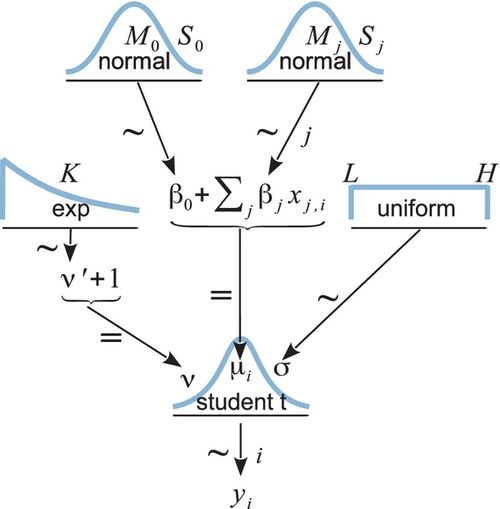
The hierarchical diagram for multiple linear regression is shown in Figure 18.4. It is merely a direct expansion of the diagram for simple linear regression in Figure 17.2 (p. 480). Instead of only one slope coefficient for a single predictor, there are distinct slope coefficients for the multiple predictors. For every coefficient, the prior is normal, just as shown in Figure 17.2. The model also uses a t distribution to describe the noise around the linear predicted value. This heavy-tailed t distribution accommodates outliers, as was described at length in Section 16.2 and subsequent sections. This model is therefore sometimes referred to as robust multiple linear regression.
As with the model for simple linear regression, the Markov Chain Monte Carlo (MCMC) sampling can be more efficient if the data are mean-centered or standardized. Now, however, there are multiple predictors to be standardized. To understand the code for standardizing the data (shown below), note that the predictor values are sent into JAGS as a matrix named x that has a column for each predictor and a row foreach data point. The data block of the JAGS code then standardizes the predictors by looping through the columns of the x matrix, as follows:
The model uses the standardized data, zx and zy, to generate credible values for the standardized parameters. The standardized parameters are then transformed to the original scale by generalizing Equation 17.2 (p. 485) to multiple predictors:

The estimate of σy is merely σzySDy, as was the case for single-predictor linear regression.
As usual, the model specification has a line of code corresponding to every arrow in the hierarchical diagram of Figure 18.4. The JAGS model specification looks like this:
The prior on the standardized regression coefficients, zbeta[j], uses an arbitrary standard deviation of 2.0. This value was chosen because standardized regression coefficients are algebraically constrained to fall between − 1 and +1 in least-squares regression, and therefore, the regression coefficients will not exceed those limits by much. A normal distribution with standard deviation of 2.0 is reasonably flat over the range from −1 to +1. The complete program is in the file Jags-Ymet-XmetMulti-Mrobust.R and a high-level script that calls it is the file Jags-Ymet-XmetMulti-Mrobust-Example.R.
18.1.3 The posterior distribution
Figure 18.5 shows the posterior distribution from the SAT data in Figure 18.3 and model in Figure 18.4. You can see that the slope on spending (Spend) is credibly above zero, even taking into account a modest ![]() OPE and MCMC instability. The slope on spending has a mode of about 13, which suggests that SAT scores rise by about 13 points for every extra $1000 spent per pupil. The slope on percentage taking the exam (PrcntTake) is also credibly non-zero, with a mode around −2.8, which suggests that SAT scores fall by about 2.8 points for every additional 1% of students who take the test.
OPE and MCMC instability. The slope on spending has a mode of about 13, which suggests that SAT scores rise by about 13 points for every extra $1000 spent per pupil. The slope on percentage taking the exam (PrcntTake) is also credibly non-zero, with a mode around −2.8, which suggests that SAT scores fall by about 2.8 points for every additional 1% of students who take the test.
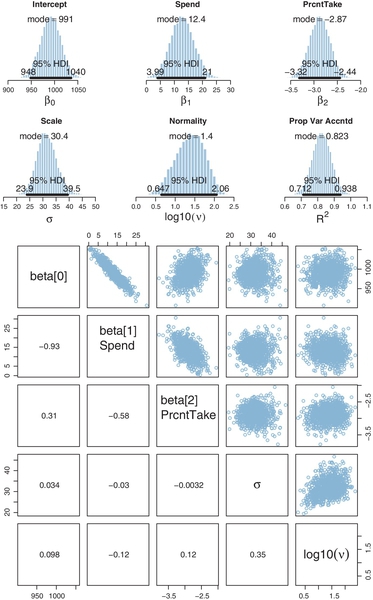
The scatter plots in the bottom of Figure 18.5 show correlations among the credible parameter values in the posterior distribution. (These are pairwise scatter plots of credible parameter values from the MCMC chain; these are not scatter plots of data.) In particular, the coefficient for spending (Spend) trades off with the coefficient on percentage taking the exam (PrcntTake). The correlation means that if we believe that the influence of spending is smaller, then we must believe that the influence of percentage taking is larger. This makes sense because those two predictors are correlated in the data.
Figure 18.5 shows that the normality parameter for these data is fairly large, suggesting that there are not many outliers for this particular selection of predictors. It is worth noting that values of y are not inherently outliers or nonoutliers; they are only outliers relative to a spread of predicted values for a particular model. A value of y that seems spurious according to one set of predictors might be nicely linearly predicted by other predictors.
Finally, Figure 18.5 also shows a posterior distribution for a statistic labeled ![]() , which is called the proportion of variance accounted for in traditional least-squares multiple regression. In least-squares regression, the overall variance in y is algebraically decomposed into the variance of the linearly predicted values and the residual variance:
, which is called the proportion of variance accounted for in traditional least-squares multiple regression. In least-squares regression, the overall variance in y is algebraically decomposed into the variance of the linearly predicted values and the residual variance: ![]() , where
, where ![]() is the linearly predicted value of yi. The proportion of variance accounted for is
is the linearly predicted value of yi. The proportion of variance accounted for is ![]() when
when ![]() is the linear prediction using coefficients that minimize
is the linear prediction using coefficients that minimize ![]() . If that makes no sense to you because you have no previous experience with least-squares regression, do not worry, because in Bayesian analysis no such decomposition of variance occurs. But for people familiar with least-squares notions who crave a statistic analogous to
. If that makes no sense to you because you have no previous experience with least-squares regression, do not worry, because in Bayesian analysis no such decomposition of variance occurs. But for people familiar with least-squares notions who crave a statistic analogous to ![]() , we can compute a surrogate. At each step in the MCMC chain, a credible value of
, we can compute a surrogate. At each step in the MCMC chain, a credible value of ![]() is computed as
is computed as ![]() , where ζj is the standardized regression coefficient for the jth predictor at that step in the MCMC chain, and ry,xj is the correlation of the predicted values, y, with the jth predictor values, xj. These correlations are constants, fixed by the data. The equation for expressing
, where ζj is the standardized regression coefficient for the jth predictor at that step in the MCMC chain, and ry,xj is the correlation of the predicted values, y, with the jth predictor values, xj. These correlations are constants, fixed by the data. The equation for expressing ![]() in terms of the regression coefficients is used merely by analogy to least-squares regression, in which the equation is exactly true (e.g., Hays, 1994, Equation 15.14.2, p. 697). The mean value in the distribution of
in terms of the regression coefficients is used merely by analogy to least-squares regression, in which the equation is exactly true (e.g., Hays, 1994, Equation 15.14.2, p. 697). The mean value in the distribution of ![]() , when using vague priors, is essentially the least-squares estimate and the maximum-likelihood estimate when using a normal likelihood function. The posterior distribution reveals the entire distribution of credible
, when using vague priors, is essentially the least-squares estimate and the maximum-likelihood estimate when using a normal likelihood function. The posterior distribution reveals the entire distribution of credible ![]() values. The posterior distribution of
values. The posterior distribution of ![]() , defined this way, can exceed 1.0 or fall below 0.0, because
, defined this way, can exceed 1.0 or fall below 0.0, because ![]() here is a linear combination of credible regression coefficients, not the singular value that minimizes the squared deviations between predictions and data.
here is a linear combination of credible regression coefficients, not the singular value that minimizes the squared deviations between predictions and data.
Sometimes we are interested in using the linear model to predict y values for x values of interest. It is straight forward to generate a large sample of credible y values for specified x values. At each step in the MCMC chain, the combination of credible parameter values is inserted into the model and random y values are generated. From the distribution of y values, we can compute the mean and highest density interval (HDI) to summarize the centrally predicted y value and the uncertainty of the prediction. As was the case for simple linear regression, illustrated back in Figure 17.3 (p. 481), the uncertainty in predicted y is greater for x values outside the bulk of the data. In other words, extrapolation is more uncertain than interpolation.
18.1.4 Redundant predictors
As a simplified example of correlated predictors, think of just two data points: Suppose y = 1 for 〈x1, x2〉 = 〈1, 1〉 and y = 2 for 〈x1, x2〉 = 〈2, 2〉. The linear model, y = β1x1 + β2x2, is supposed to satisfy both data points, and in this case both are satisfied by 1 = β1 + β2. Therefore, many different combinations of β1 and β2 satisfy the data. For example, it could be that β1 = 2 and β2 = −1, or β1 = 0.5 and β2 = 0.5, or β1 = 0 and β2 = 1. In other words, the credible values of β1 and β2 are anticorrelated and trade-off to fit the data.
One of the benefits of Bayesian analysis is that correlations of credible parameter values are explicit in the posterior distribution. Another benefit of Bayesian analysis is that the estimation doesn't “explode” when predictors are strongly correlated. If predictors are correlated, the joint uncertainty in the regression coefficients is evident in the posterior, but the analysis happily generates a posterior distribution regardless of correlations in the predictors. In extreme cases, when the predictors are very strongly correlated, the marginal posteriors will simply reflect the prior distributions on the regression coefficients, with a strong trade-off in their joint posterior distribution.
For illustration, we will use a completely redundant predictor, namely the proportion of students not taking the exam. Thus, if PrcntTake is the percentage of students taking the exam, then PropNotTake = (100 − PrcntTake)/100 is the proportion of students not taking the exam. For example, if PrcntTake = 37, then PropNotTake = 0.63. These sorts of redundant predictors can show up in real analyses. Sometimes, the redundant predictors are included because the analyst does not realize (initially) that they are redundant, perhaps because the predictors are labeled differently and come from different sources and are on seemingly different scales. Other times, the predictors are not inherently redundant, but happen to be extremely strongly correlated in the data. For example, suppose we use temperature as a predictor, and we measure the temperature with two thermometers sitting side by side. Their readings should be almost perfectly correlated, even if one has a Celsius scale and the other has a Fahrenheit scale.
Figure 18.6 shows the posterior distribution. One sign of redundant predictors is the (very nearly) perfect correlation between the credible values of the slopes on the predictors, revealed in the pairwise scatter plots. Because the predictors are redundant, the credible regression coefficients trade-off with each other but still fit the data equally well. Consequently, the marginal posterior distribution of either predictor is extremely broad, as can be seen in the upper panels of Figure 18.6. Thus, an extremely broad marginal posterior distribution is another clue that there might be redundancies in the predictors.

Another important clue to redundancy in predictors is autocorrelation in the MCMC chains for the regression coefficients of the predictors. When you run the script, you will see that diagnostic graphs of the chains are generated (not shown here). The chains for the regression coefficients of redundant predictors are highly autocorrelated and very highly correlated with each other.
Unfortunately, the signs of predictor redundancy in the posterior distribution get diffused when there are three of more strongly correlated predictors. In particular, the pairwise scatter plots are not sufficient to show a three-way trade-off of regression coefficients. Autocorrelation remains high, however.
Of course, the most obvious indicator of redundancy in predictors is not in the posterior distribution of the regression coefficients, but in the predictors themselves. At the beginning of the program, the correlations of the predictors are displayed in the ![]() console, like this:
console, like this:
If any of the nondiagonal correlations are high (i.e., close to +1 or close to −1), be careful when interpretingthe posteriordistribution. Here, we can see that the correlation of PrcntTake and PropNotTake is −1.0, which is an immediate sign of redundant predictors.
Traditional methods for multiple linear regression can break down when predictors are perfectly (or very strongly) correlated because there is not a unique solution for the best fitting parameter values. Bayesian estimation has no inherent problems with such cases. The posterior distribution merely reveals the trade-off in the parameters and the resulting large uncertainty in their individual values. The extent of the uncertainty is strongly influenced by the prior distribution in this case, because there is potentially an infinite trade-off among equally well-fitting parameter values, and only the prior distribution tempers the infinite range of possibilities. Figure 18.7 shows the prior distribution for this example, transformed to the original scale of the data.2 Notice that the posterior distribution in Figure 18.6 has ranges for the redundant parameters that are only a little smaller than their priors. If the priors were wider, the posteriors on the redundant parameters would also be wider.

What should you do if you discover redundant predictors? If the predictors are perfectly correlated, then you can simply drop all but one, because the predictors are providing identical information. In this case, retain the predictor that is most relevant for interpreting the results. If the predictors are not perfectly correlated, but very strongly correlated, then there are various options directed at extracting an underlying common factor for the correlated predictors. One option is arbitrarily to create a single predictor that averages the correlated predictors. Essentially, each predictor is standardized, inverted as appropriate so that the standardized values have positive correlation, and then the average of the standardized values is used as the unitary predictor that represents all of the correlated predictors. More elaborate variations of this approach use principal components analysis. Finally, instead of creating a deterministic transform of the predictors, an underlying common factor can be estimated using factor analysis or structural equation modeling (SEM). These methods can be implemented in Bayesian software, of course, but go beyond the intended scope of this book. For an introduction to SEM in BUGS (hence easily convertible to JAGS and Stan), see the article by Song and Lee (2012). Another introductory example of Bayesian SEM is presented by Zyphur and Oswald (2013) but using the proprietary software Mplus.
18.1.5 Informative priors, sparse data, and correlated predictors
The examples in this book tend to use mildly informed priors (e.g., using information about the rough magnitude and range of the data). But a benefit of Bayesian analysis is the potential for cumulative scientific progress by using priors that have been informed from previous research.
Informed priors can be especially useful when the amount of data is small compared to the parameter space. A strongly informed prior essentially reduces the scope of the credible parameter space, so that a small amount of new data implies a narrow zone of credible parameter values. For example, suppose we flip a coin once and observe a head. If the prior distribution on the underlying probability of heads is vague, then the single datum leaves us with a broad, uncertain posterior distribution. But suppose we haveprior knowledge that the coin is manufactured by a toy company that creates trick coins that either always come up heads or always come up tails. This knowledge constitutes a strongly informed prior distribution on the underlying probability of heads, with a spike of 50% mass at zero (always tails) and a spike of 50% mass at one (always heads). With this strong prior, the single datum yields a posterior distribution with complete certainty: 100% mass at one (always heads).
As another example of using strong prior information with sparse data, recall the linear regression of weight on height for 30 people in Figure 17.3 (p. 481). The marginal posterior distribution on the slope has a mode of about 4.5 and a fairly broad 95% HDI that extends from about 2.0 to 7.0. Furthermore, the joint posterior distribution on the slope and intercept shows a strong trade-off, illustrated in the scatter plot of the MCMC chain in Figure 17.3. For example, if the slope is about 1.0, then credible intercepts would have to be about +100, but if the slope is about 8.0, then credible intercepts would have to be about −400. Now, suppose that we have strong prior knowledge about the intercept, namely, that a person who has zero height has zero weight. This “knowledge” might seem to be a logical truism, but actually it does not make much sense because the example is referring to adults, none of whom have zero height. But we will ignore reality for this illustration and suppose that we know the intercept must be at zero. From the trade-off in credible intercepts and slopes, an intercept of zero implies that the slope must be very nearly 2.0. Thus, instead of a broad posterior distribution on the slopes that is centered near 4.5, the strong prior on the intercept implies a very narrow posterior distribution on the slopes that is centered near 2.0.
In the context of multiple linear regression, sparse data can lead to usefully precise posteriors on regression coefficients if some of the regression coefficients have informed priors and the predictors are strongly correlated. To understand this idea, it is important to remember that when predictors are correlated, their regression coefficients are also (anti-)correlated. For example, recall the SAT data from Figure 18.3 (p. 514) in which spending-per-pupil and percent-taking-the-exam are correlated. Consequently, the posterior estimates of the regression coefficients had a negative correlation, as shown in Figure 18.5 (p. 518). The correlation of credible regression coefficients implies that a strong belief about the value of one regression coefficient constrains the value of the other coefficient. Look carefully at the scatter plot of the two slopes shown in Figure 18.5. It can be seen that if we believe that the slope on percent-taking-the-exam is −3.2, then credible values of the slope on spending-per-pupil must be around 15, with an HDI extending roughly from 10 to 20. Notice that this HDI is smaller than the marginal HDI on spending-per-pupil, which goes from roughly 4 to 21. Thus, constraining the possibilities of one slope also constrains credible values of the other slope, because estimates of the two slopes are correlated.
That influence of one slope estimate on another can be used for inferential advantage when we have prior knowledge about one of the slopes. If some previous or auxiliaryresearch informs the prior of one regression coefficient, that constraint can propagate to the estimates of regression coefficients on other predictors that are correlated with the first. This is especially useful when the sample size is small, and a merely mildly informed prior would not yield a very precise posterior. Of course, the informed prior on the first coefficient must be cogently justified. This might not be easy, especially in the context of multiple linear regression, where the inclusion of additional predictors can greatly change the estimates of the regression coefficients when the predictors are correlated. A robustness check also may be useful, to show how strong the prior must be to draw strong conclusions. If the information used for the prior is compelling, then this technique can be very useful for leveraging novel implications from small samples. An accessible discussion and example from political science is provided by Western and Jackman (1994), and a mathematical discussion is provided by Learner (1978, p. 175+).
18.2 Multiplicative interaction of metric predictors
In some situations, the predicted value might not be an additive combination of the predictors. For example, the effects of drugs are often nonadditive. Consider the effects of two drugs, A and B. The effect of increasing the dose of drug B might be positive when the dose of drug A is small, but the effect of increasing drug B might be negative when the dose of drug A is large. Thus, the effects of the two drugs are not additive, and the effect of a drug depends on the level of the other drug. As another example, consider trying to predict subjective happiness from income and health. If health is low, then an increase in income probably has only a small effect. But if health is high, then an increase from low income to high income probably has a large effect. Thus, the effects of the two factors are not additive, and the effect of one factor depends on the level of the other factor.
Formally, interactions can have many different specific functional forms. We will consider multiplicative interaction. This means that the nonadditive interaction is expressed by multiplying the predictors. The predicted value is a weighted combination of the individual predictors and, additionally, the multiplicative product of the predictors. For two metric predictors, regression with multiplicative interaction has these algebraically equivalent expressions:


These three expressions emphasize different interpretations of interaction, as illustrated in Figure 18.8. The form of Equation 18.2 is illustrated in the left panel of Figure 18.8. The vertical arrows show that the curved-surface interaction is created by adding the product, β1×2x1x2, to the planar linear combination.

The form of Equation 18.3 is illustrated in the middle panel of Figure 18.8. Its dark lines show that the slope in the x1 direction depends on the value of x2. In particular, when x2 = 0, then the slope along x1 is β1 + β1×2x2 = −1 + 0.2 · 0 = − 1. But when x2 = 10, then the slope along x1 is β1 + β1×2x2 = −1 + 0.2 · 10 = + 1. Again, the slope in the x1 direction changes when x2 changes, and β1 only indicates the slope along x1 when x2 = 0.
The form of Equation 18.4 is illustrated in the right panel of Figure 18.8. It shows that the interaction can be expressed as the slope in the x2 direction changing when x1 changes. (Exercise 18.1 has you compute the numerical slopes.) This illustration is exactly analogous to the middle panel of Figure 18.8, but with the roles of x1 and x2 exchanged. It is important to realize, and visualize, that the interaction can be expressed in terms of the slopes on either predictor.
Great care must be taken when interpreting the coefficients of a model that includes interaction terms (Braumoeller, 2004). In particular, low-order terms are especially difficult to interpret when higher-order interactions are present. In the simple two-predictor case, the coefficient β1 describes the influence of predictor x1only at x2 = 0, because the slope on x1 is β1 + β1×2x2, as was shown in Equation 18.3 and graphed in the middle panel of Figure 18.8. In other words, it is not appropriate to say that β1 indicates the overall influence of x1 on y. Indeed, in many applications, the value of x2never realistically gets close to zero, and therefore, β1 has no realistic interpretation at all. For example, suppose we are predicting college GPA (y) from parental income (x1) and high-school GPA (x2). If there is interaction, then the regression coefficient, β1, on parental income, only indicates the slope on x1when x2(GPA) is zero. Of course, there are no GPAs of zero, and therefore, β1 by itself is not very informative.
18.2.1 An example
To estimate the parameters of a model with multiplicative interaction, we could create a new program in JAGS or Stan that takes the unique predictors as input and then multiplies them internally for the desired interactions. This approach would be conceptually faithful because it maintains the idea that there are two predictors and the model combines them nonadditively. But instead of creating a new program, we will use the previously applied additive (noninteraction) model by inventing another predictor that expresses the product of the individual predictors. To do this, we conceptualize the interaction term of Equation 18.2 as an additional additive predictor, like this:
We create the new variable x3 = x1x2 outside the model and then submit the new variable as if it were another additive predictor. One benefit of this approach is that we do not have to create a new model, and it is easy, in cases of many predictors, to set up interaction variables for many different combinations of variables. Another key benefit is that we can examine the correlations of the single predictors with the interaction variables. Often the single variables will be correlated with the interaction variables, and therefore, we can anticipate trade-offs in the estimated parameter values that widen the marginal posterior distributions on single parameters.
To illustrate some of the issues involved in interpreting the parameters of a model with interaction, consider again the SAT data from Figure 18.3. ![]() ecall that the mean SAT score in a state was predicted from the spending per pupil (Spend) and the percentage of students who took the test (PrcntTake). When no interaction term was included in the model, the posterior distribution looked like Figure 18.5, which indicated a positive influence of Spend and a negative influence of PrcntTake.
ecall that the mean SAT score in a state was predicted from the spending per pupil (Spend) and the percentage of students who took the test (PrcntTake). When no interaction term was included in the model, the posterior distribution looked like Figure 18.5, which indicated a positive influence of Spend and a negative influence of PrcntTake.
We will include a multiplicative interaction of Spend and PrcntTake. Does it make sense that the effect of spending might depend on the percentage of students taking the test? Perhaps yes, because if very few students are taking the test, they are probably already at the top of the class and therefore might not have as much head-room for increasing their scores if more money is spent on them. In other words, it is plausible that the effect of spending is larger when the percentage of students taking the test islarger, and we would not be surprised if there were a positive interaction between those predictors. Therefore, it is theoretically meaningful to include an interaction term in the model.
The computer code for this example is in one of the sections of the file Jags-Ymet-XmetMulti-Mrobust-Example.R. The commands read the data and then create a new variable that is appended as another column on the data frame, after which the relevant column names are specified for the analysis:
When the analysis is run, the first thing it does is display the correlations of the predictors:
We can see that the interaction variable is strongly correlated with both predictors. Therefore, we know that there will be strong trade-offs among the regression coefficients, and the marginal distributions of single regression coefficients might be much wider than when there was no interaction included.
When we incorporate a multiplicative interaction into the model, the posterior looks like Figure 18.9. The marginal distribution for β3, also labeled as SpendXPrcnt, indicates that the modal value of the interaction coefficients is indeed positive, as we anticipated it could be. However, the 95% HDI includes zero, which indicates that we do not have very strong precision in the estimate of the magnitude of the interaction.

Notice that the inclusion of the interaction term has changed the apparent marginal distributions for the regression coefficients on Spend and PrcntTake. In particular, the regression coefficient on Spend now clearly includes zero. This might lead a person, inappropriately, to conclude that there is not a credible influence of spending on SAT scores, because zero is among the credible values of β1. This conclusion is not appropriate because β1 only indicates the slope on spending when the percentage of students taking the test is zero. The slope on Spend depends on the value of PrcntTake because of the interaction.
To properly understand the credible slopes on the two predictors, we must consider the credible slopes on each predictor as a function of the value of the other predictor. ![]() ecall from Equations 18.3 that the slope on x1 is β1 + β1×2x2. Thus, for the present application, the slope on Spend is β1 + β3 · PrcntTake because β1×2 is β3 and x2 is PrcntTake. Thus, for any particular value of PrcntTake, we get the distribution of credible slopes on Spend by stepping through the MCMC chain and computing β1 + β3 · PrcntTake at each step. We can summarize the distribution of slopes by its median and 95% HDI. We do that for many candidate values of PrcntTake, and the result is plotted in the middle panel of Figure 18.9. You can see that when PrcntTake is large, the credible slopes on Spend clearly exceed zero. You can also mentally extrapolate that when PrcntTake is zero, the median and HDI will match the marginal distribution of β1 shown in the top of Figure 18.9.
ecall from Equations 18.3 that the slope on x1 is β1 + β1×2x2. Thus, for the present application, the slope on Spend is β1 + β3 · PrcntTake because β1×2 is β3 and x2 is PrcntTake. Thus, for any particular value of PrcntTake, we get the distribution of credible slopes on Spend by stepping through the MCMC chain and computing β1 + β3 · PrcntTake at each step. We can summarize the distribution of slopes by its median and 95% HDI. We do that for many candidate values of PrcntTake, and the result is plotted in the middle panel of Figure 18.9. You can see that when PrcntTake is large, the credible slopes on Spend clearly exceed zero. You can also mentally extrapolate that when PrcntTake is zero, the median and HDI will match the marginal distribution of β1 shown in the top of Figure 18.9.
The bottom panel of Figure 18.9 shows the credible slopes on PrcntTake for particular values of Spend. At each step in the MCMC chain, a credible slope was computed as β2 + β3 · Spend. You can see that the median slope on PrcntTake is not constant but depends on the value of Spend. This dependency of the effect of one predictor on the level of the other predictor is the meaning of interaction.
In summary, when there is interaction, then the influence of the individual predictors can not be summarized by their individual regression coefficients alone, because those coefficients only describe the influence when the other variables are at zero. A careful analyst considers credible slopes across a variety of values for the other predictors, as in Figure 18.9. Notice that this is true even though the interaction coefficient did not exclude zero from its 95% HDI. In other words, if you include an interaction term, you cannot ignore it even if its marginal posterior distribution includes zero.
18.3 Shrinkage of regression coefficients
In some research, there are many candidate predictors which we suspect could possibly be informative about the predicted variable. For example, when predicting college GPA, we might include high-school GPA, high-school SAT score, income of student, income of parents, years of education of the parents, spending per pupil at the student's high school, student IQ, student height, weight, shoe size, hours of sleep per night, distance from home to school, amount of caffeine consumed, hours spent studying, hours spent earning a wage, blood pressure, etc. We can include all the candidate predictors in the model, with a regression coefficient for every predictor. And this is not even considering interactions, which we will ignore for now.
With so many candidate predictors of noisy data, there may be some regression coefficients that are spuriously estimated to be non-zero. We would like some protection against accidentally nonzero regression coefficients. Moreover, if we are interested in explaining variation in the predicted variable, we would like the description of the data to emphasize the predictors that are most clearly related tovariable. In other words, we would like the description to de-emphasize weak or spurious predictors.
One way to implement such a description is by using a t distribution for the prior on the regression coefficients. By setting its mean to zero, its normality parameter to a small value, and its scale parameter to a moderately small value, the t-distributed prior dictates that regression coefficients should probably be near zero, where the narrow peak of the t distribution is. But if a regression coefficient is clearly nonzero, then it could be large, as is allowed by the heavy tail of the t-distributed prior.
Figure 18.10 shows a diagram of a multiple linear regression model that has a t-distributed prior on the regression coefficients. Compare the diagram with the one in Figure 18.4 (p. 515), and you will see that the only difference from before is the prior on the regression coefficients. The empty braces in the top of Figure 18.10 refer to optional aspects of the model. As was mentioned in the previous paragraph, the normality parameter νβ and the scale parameter σβ could be set to constants, in which case the braces as the top of the diagram would enclose constants and the arrows would be labeled with an equal sign. When the prior has constants, it is sometimes called a regularizer for the estimation.
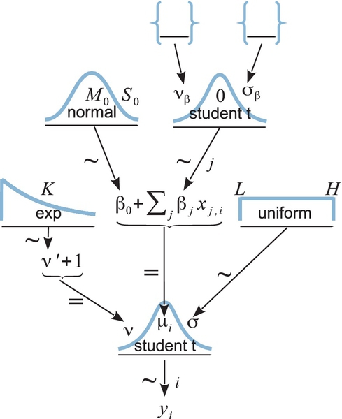
The t-distributed prior is just one way to express the notion that regression coefficients near zero should be preferred but with larger coefficients allowed. Alternatively, a double exponential distribution could be used. A double exponential is simply an exponential distribution on both +β and −β, equally spread. The double exponential has a single-scale parameter (and no shape parameter). The double exponential is built into JAGS and Stan. A well-known regularization method called lasso regression uses a double exponential weighting on the regression coefficients. For a nice explanation of lasso regression in a Bayesian setting, see Lykou and Ntzoufras (2011).
Should the scale parameter (i.e., σβ in Figure 18.10) be fixed at a constant value or should it be estimated from the data? If it is fixed, then every regression coefficient experiences the same fixed regularization, independently from all the other regression coefficients. If the scale parameter is estimated, then the variability of the estimated regression coefficients across predictors influences the estimate of the scale parameter, which in turn influences all the regression coefficients. In particular, if most of the regression coefficients are estimated to be near zero, then the scale parameter is estimated to be small, which further shrinks the estimates of the regression coefficients.
Neither one of these approaches (using fixed σβ or estimated σβ) is inherently “correct.” The approaches express different prior assumptions. If the model estimates σβ (instead of fixing it), the model is assuming that all the regression coefficients are mutually representative of the variability across regression coefficients. In applications where there are many predictors of comparable status, this assumption may be quite realistic. A minimal requirement, for putting all the regression coefficients under a shared overarching distribution with an estimated scale, is that the predictors were selected from some implicit set of reasonably likely predictors, and therefore, we can think of the overarching distribution as reflecting that set. In applications where there are relatively few predictors of different types, this assumption might not be appropriate. Beware of convenience priors that are used in routinized ways.
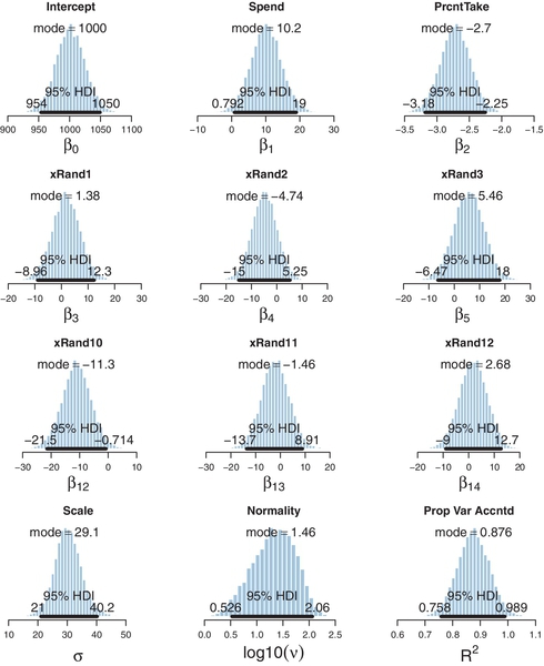
To illustrate these ideas with a concrete example, consider again the SAT data of Figure 18.3, but now supplemented with 12 more randomly generated predictors. The x values were randomly and independently drawn from a normal distribution centered at zero, and therefore, any correlation between the predictors and any nonzero regression coefficient is an accident of random sampling. We will first apply the simple model of Figure 18.4, for which the regression coefficients have fixed, independent, vague normal priors. The resulting posterior distribution is shown in Figure 18.11. To save space, the results for random predictors 4-9 (x![]() and4–x
and4–x![]() and9) have not been displayed. Attend specifically to the distributions for the regression coefficients on spending (Spend) and random predictor 10 (x
and9) have not been displayed. Attend specifically to the distributions for the regression coefficients on spending (Spend) and random predictor 10 (x![]() and10). The coefficient on Spend is still estimated to be positive and its 95% HDI falls above zero, but only barely. The inclusion of additional predictors and their parameters has reduced the certainty of the estimate. The coefficient on x
and10). The coefficient on Spend is still estimated to be positive and its 95% HDI falls above zero, but only barely. The inclusion of additional predictors and their parameters has reduced the certainty of the estimate. The coefficient on x![]() and10 is negative, with its 95% HDI falling below zero, to about the same extent as Spend fell above zero. This apparent relation of x
and10 is negative, with its 95% HDI falling below zero, to about the same extent as Spend fell above zero. This apparent relation of x![]() and10 with SAT score is spurious, an accident of random sampling. We know that the apparently nonzero relation of x
and10 with SAT score is spurious, an accident of random sampling. We know that the apparently nonzero relation of x![]() and10 with SAT score is spurious only because we generated the data. For data collected from nature, such as spending and SAT scores, we cannot know which estimates are spurious and which are genuine. Bayesian analysis tells us the best inference we can make, given the data and our choice of descriptive model.
and10 with SAT score is spurious only because we generated the data. For data collected from nature, such as spending and SAT scores, we cannot know which estimates are spurious and which are genuine. Bayesian analysis tells us the best inference we can make, given the data and our choice of descriptive model.
Now we repeat the analysis using the hierarchical model of Figure 18.10, with νβ fixed at one (i.e., heavy tails), and with σβ given a gamma prior that has mode 1.0 and standard deviation 1.0 (i.e., broad for the standardized data). The programs for this analysis are in files Jags-Ymet-XmetMulti-MrobustShrink.R and Jags-Ymet-XmetMulti-MrobustShrink-Example.R. The resulting posterior distribution is shown in Figure 18.12. Notice that the marginal distribution for the regression coefficient on x![]() and10 is now shifted so that its 95% HDI covers zero. The estimate is shrunken toward zero because many predictors are telling the higher-level t distribution that their regression coefficients are near zero. Indeed, the estimate of σβ (not displayed) has its posterior mode around 0.05, even though its prior mode was at 1.0. The shrinkage also causes the estimate of the regression coefficient on Spend to shift toward zero. Thus, the shrinkage has suppressed a spurious regression coefficient on x
and10 is now shifted so that its 95% HDI covers zero. The estimate is shrunken toward zero because many predictors are telling the higher-level t distribution that their regression coefficients are near zero. Indeed, the estimate of σβ (not displayed) has its posterior mode around 0.05, even though its prior mode was at 1.0. The shrinkage also causes the estimate of the regression coefficient on Spend to shift toward zero. Thus, the shrinkage has suppressed a spurious regression coefficient on x![]() and10, but it has also suppressed what might be a real but small regression coefficient on Spend. Notice, however, that the marginal distribution for the coefficient on PrcntTake has not been much affected by shrinkage, presumably because it is big enough that it falls in the tail of the t distribution where the prior is relatively flat.
and10, but it has also suppressed what might be a real but small regression coefficient on Spend. Notice, however, that the marginal distribution for the coefficient on PrcntTake has not been much affected by shrinkage, presumably because it is big enough that it falls in the tail of the t distribution where the prior is relatively flat.

The shrinkage is desirable not only because it shares information across predictors (as expressed by the hierarchical prior) but also because it rationally helps control for false alarms in declaring that a predictor has a nonzero regression coefficient. As the example in Figure 18.11 showed, when there are many candidate predictors, some of them may spuriously appear to have credibly nonzero regression coefficients even when their true coefficients are zero. This sort of false alarm is unavoidable because data are randomly sampled, and there will be occasional coincidences of data that are unrepresentative. By letting each regression coefficient be informed by the other predictors, the coefficients are less likely to be spuriously distorted by a rogue sample.
Finally, notice in Figure 18.12 that the marginal posterior distributions on many of the regression coefficients are (upside-down) funnel shaped, each with a pointy peak near zero and long concave tails, like this: ![]() . You can imagine that the posterior distribution from the nonshrinkage model, which is gently rounded at its peak, was pinched at a point on its top edge and lifted over toward zero, like a mommy cat carrying a kitten by the scruff of its neck back to its bed. A funnel shape is characteristic of a posterior distribution experiencing strong shrinkage. (We have previously seen examples of this, for example way back in Figure 9.10, p. 243. Another example is shown in Exercise 19.1.) If a marginal posterior distribution is displayed only by a dot at its central tendency and a segment for its HDI, without a profile for its shape, then this signature of shrinkage is missed.
. You can imagine that the posterior distribution from the nonshrinkage model, which is gently rounded at its peak, was pinched at a point on its top edge and lifted over toward zero, like a mommy cat carrying a kitten by the scruff of its neck back to its bed. A funnel shape is characteristic of a posterior distribution experiencing strong shrinkage. (We have previously seen examples of this, for example way back in Figure 9.10, p. 243. Another example is shown in Exercise 19.1.) If a marginal posterior distribution is displayed only by a dot at its central tendency and a segment for its HDI, without a profile for its shape, then this signature of shrinkage is missed.
18.4 Variable selection
The motivation of the previous section was an assumption that many predictors might have weak predictive value relative to the noise in the data, and therefore, shrinkage would be appropriate to stabilize the estimates. In some applications, it may be theoretically meaningful to suppose that a predictor has literally zero predictive value. In this case, the issue is not estimating a presumed weak predictiveness relative to noise; instead, the issue is deciding whether there is any predictiveness at all. This is almost antithetical to including the predictor in the first place, because including it means that we had some prior belief that the predictor was relevant. Nevertheless, we might want to estimate the credibility that the predictor should be included, in combination with various subsets of other predictors. Deciding which predictors to include is often called variable selection.
Some prominent authors eschew the variable-selection approach for typical applications in their fields. For example, Gelman et al. (2013, p. 369) said, “For the regressions we typically see, we do not believe any coefficients to be truly zero and we do not generally consider it a conceptual (as opposed to computational) advantage to get point estimates of zero—but regularized estimates such as obtained by lasso can be much better than those resulting from simple least squares and flat prior distributions …we are not comfortable with an underlying model in which the coefficients can be exactly zero.” Other researchers take it for granted, however, that some form of variable selection must be used to make sense of their data. For example, O’Hara and Sillanpää (2009, p. 86) said, “One clear example where this is a sensible way to proceed is in gene mapping, where it is assumed that there are only a small number of genes that have a large effect on a trait, while most of the genes have little or no effect. The underlying biology is therefore sparse: only a few factors (i.e. genes) are expected to influence the trait.” They later said, however, “In any real data set, it is unlikely that the ‘true’ regression coefficients are either zero or large; the sizes are more likely to be tapered towards zero. Hence, the problem is not one of finding the zero coefficients, but of finding those that are small enough to be insignificant, and shrinking them towards zero “(O’Hara & Sillanpää, 2009, p. 95).” Thus, we are entertaining a situation in which there are many candidate predictors that may genuinely have zero real relation to the predicted value or have relations small enough to be counted as insignificant. In this situation, a reasonable question is, which predictors can be credibly included in the descriptive model?
This section introduces some basic ideas and methods of Bayesian variable selection, using some simple illustrative examples. The topic is extensively studied and undergoing rapid development in the literature. The examples presented here are intended to reveal some of the foundational concepts and methods, not to serve as a comprehensive reference for the latest and greatest methods. After studying this section, please see the various cited references and other literature for more details.
There are various methods for Bayesian variable selection (see, e.g., O’Hara & Sillanpää, 2009; Ntzoufras, 2009). The key to models of variable selection (as opposed to shrinkage) is that each predictor has both a regression coefficient and an inclusion indicator, which can be thought of as simply another coefficient that takes on the values 0 or 1. When the inclusion indicator is 1, then the regression coefficient has its usual role. When the inclusion indicator is 0, the predictor has no role in the model and the regression coefficient is superfluous.
To formalize this idea, we modify the basic linear regression equation with a new parameter δj ∈{0,1}, which is the inclusion indicator for the jth predictor. The predicted mean value of y is then given by
Every combination of δj values, across the predictors, constitutes a distinct model of the data. For example, if there are four predictors, then ![]() is a model that includes all four predictors, and
is a model that includes all four predictors, and ![]() is a model that includes only the second and fourth predictors, and so on. With four predictors, there are 24 = 16 possible models.
is a model that includes only the second and fourth predictors, and so on. With four predictors, there are 24 = 16 possible models.
A simple way to put a prior on the inclusion indicator is to have each indicator come from an independent Bernoulli prior, such as δj∼ dbern(0.5). The constant in the prior affects the prior probability of models with more or fewer predictors included. With a prior inclusion bias of 0.5, all models are equally credible, a priori. With a prior inclusion bias less than 0.5, models with less than half the predictors included are a priori more credible than models with more than half the predictors.
It is trivial to incorporate the inclusion parameter in a JAGS model specification, as will shown presently.3 As in all the regression models we have used, the data are standardized in the initial data block of the JAGS code, which is not repeated here. ![]() ecall that the standardized data are denoted as zx[i,1:Nx], where the index i denotes the ith individual and where Nx indicates the number of predictors. The standardized regression coefficients are denoted as zbeta[1:Nx], and the new inclusion indicators are denoted as delta[1:Nx]. The model specification (which you may compare with the model specification in Section 18.1.2, p. 514) is as follows:
ecall that the standardized data are denoted as zx[i,1:Nx], where the index i denotes the ith individual and where Nx indicates the number of predictors. The standardized regression coefficients are denoted as zbeta[1:Nx], and the new inclusion indicators are denoted as delta[1:Nx]. The model specification (which you may compare with the model specification in Section 18.1.2, p. 514) is as follows:
There are only three lines above that use the new inclusion parameter. The first usage is in the specification of the likelihood for zy[i]. Instead of the predicted mean involving sum(zbeta[1:Nx] * zx[i,1:Nx] ),it uses sum( delta[1:Nx] * zbeta[1:Nx] * zx[i,1:Nx] ). The second appearance of the inclusion parameter is the specification of its Bernoulli prior. Finally, near the end of the specification above, the transformation from standardized to original scale also incorporates the inclusion indicators. This is necessary because zbeta[j] is irrelevant when it is not used to model the data.
As a first example of applying the variable-selection method, recall the SAT data of Figure 18.3 and the posterior distribution shown in Figure 18.5. For each of 50 states, the average SAT score was regressed on two predictors: average spending per pupil (Spend) and percentage of students who took the test (PrcntTake). With two predictors, there are four possible models involving different subsets of predictors. Because the prior inclusion probability was set at 0.5, each model had a prior probability of 0.52 = 0.25.
Figure 18.13 shows the results. Of the four possible models, only two had a non-negligible posterior probability, namely the model that included both predictors and the model that included only PrcntTake. As shown in the upper panel of Figure 18.13, the model with both predictors has a posterior probability of about 70%. This value is simply the number of times that the MCMC chain had ![]() divided by the total number of steps in the chain. Like any MCMC estimate, it is based on a random sample and will be somewhat different on different runs. As shown in the lower panel of Figure 18.13, the model with only PrcntTake has a posterior probability of about 30%. This value is simply the number of times that the MCMC chain had
divided by the total number of steps in the chain. Like any MCMC estimate, it is based on a random sample and will be somewhat different on different runs. As shown in the lower panel of Figure 18.13, the model with only PrcntTake has a posterior probability of about 30%. This value is simply the number of times that the MCMC chain had ![]() divided by the total number of steps in the chain. Thus, the model involving both predictors is more than twice as credible as the model involving only one predictor.
divided by the total number of steps in the chain. Thus, the model involving both predictors is more than twice as credible as the model involving only one predictor.

Figure 18.13 also shows the marginal posterior distributions of the included regression coefficients. These are credible values taken only from the corresponding steps in the chain. Thus, the histograms in the upper panel involve only ≈70% of the chain for which ![]() , and the histograms in the lower panel involve only the ≈30% of the chain for which
, and the histograms in the lower panel involve only the ≈30% of the chain for which ![]() . Notice that the parameter estimates are different for different models. For example, the estimate of the intercept is quite different for different included predictors.
. Notice that the parameter estimates are different for different models. For example, the estimate of the intercept is quite different for different included predictors.
18.4.1 Inclusion probability is strongly affected by vagueness of prior
We will now see that the degree of vagueness of the prior on the regression coefficient can have an enormous influence on the inclusion probability, even though the degree of vagueness has little influence on the estimate of the regression coefficient itself. ![]() ecall that the prior in the model was specified as a generic broad distribution on the standardized regression coefficients, like this:
ecall that the prior in the model was specified as a generic broad distribution on the standardized regression coefficients, like this:
The choice of SD=2 was arbitrary but reasonable because standardized regression coefficients cannot exceed ±1 in least-squares regression. When running the model on the SAT data with two candidate predictors, the result was shown in Figure 18.13 (p. 539).
We now re-run the analysis using different arbitrary degrees of vagueness on the priors for the standardized regression coefficients. We will illustrate with SD=1,like this:
and with SD=10,like this:
Notice that the prior probability on the inclusion parameters has not changed. The prior inclusion probability is always 0.5 in these examples.
Figure 18.14 shows the results. The upper pair of panels shows the posterior probabilities when the prior on the standardized regression coefficients has SD=1. You can see that there is a strong advantage for the two-predictor model, with the posterior inclusion probability of Spend being about 0.82The lower pair of panels in Figure 18.14 shows the posterior probabilities when the prior on the standardized regression coefficients has SD=10. You can see that there is now an advantage for the one-predictor model, with the posterior inclusion probability of Spend being only about 0.36. How could that be? After all, a model with all predictors included must be able to fit the data at least as well as a model with only a subset of predictors excluded.

The reason for the lower probability of the more complex model is that each extra parameter dilutes the prior density on the pre-existing parameters. This idea was discussed in Section 10.5 (p. 289). Consider the PrcntTake-only model. In this model, one of the most credible values for the regression coefficient on PrcntTake is β2 = −2.5. The likelihood at that point involves p(D|β2 = −2.5) and the prior density at the point involves p(β2 =−2.5), with the posterior probability proportional to their product. The very same likelihood can be achieved by the model that also includes Spend, merely by setting the regression coefficient on Spend to zero: p(D|β2 = −2.5) = p(D|β2= −2.5, β1 = 0). But the prior density at that point, p(β2 = −2.5, β1 = 0) = p(β2 = −2.5) p(β1 = 0), will typically be less than p(β2 = −2.5), because the prior is p(β2 = −2.5) multiplied by a probability density that is almost certainly less than one. Thus, models that include more predictors will pay the cost of lower prior probability. Models with additional predictors will be favored only to the extent that their benefit in higher likelihood outweighs their cost in lower prior probability. When the prior on the regression coefficient is broader, the prior density at any particular value tends to get smaller.
On the other hand, the change in vagueness of the prior distribution has hardly affected the estimates of the regression coefficients at all. Figure 18.14 shows that the estimate of the regression coefficient on Spend has a 95% HDI from about 4 to 21 for both prior distributions, regardless of whether its inclusion probability is low or high. From these results, do we conclude that Spend should be included or not? For me, the robustness of the explicit estimate of the regression coefficient, showing that it is nonzero, trumps the model comparison. As has been emphasized previously in Section 10.6 (p. 292) and in Section 12.4 (p. 354), Bayesian model comparison can be strongly affected by the degree of vagueness in the priors, even though explicit estimates of the parameter values may be minimally affected. Therefore, be very cautious when interpreting the results of Bayesian variable selection. The next section discusses a way to inform the prior by using concurrent data instead of previous data.
18.4.2 Variable selection with hierarchical shrinkage
The previous section emphasized the importance of using appropriate priors on the regression coefficients when doing variable selection, because the vagueness of the priors can have surprisingly large influence on the posterior inclusion probabilities. If you have strong previous research that can inform the prior, then it should be used. But if previous knowledge is weak, then the uncertainty should be expressed in the prior. This is an underlying mantra of the Bayesian approach: Any uncertainty should be expressed in the prior. Thus, if you are not sure what the value of σβ should be, you can estimate it and include a higher-level distribution to express your prior uncertainty. In other words, in Figure 18.10 (p. 531), we estimate σβ and give it a prior distribution in place of the open braces. An additional benefit of this approach is that all the predictors simultaneously inform the estimate of σβ, whereby concurrent data from all the predictors provide an informed prior for each individual predictor.
In the present application, we have uncertainty, and therefore, we place a broad prior on σβ. The code below shows a few different options in commented lines. In the code, σβ is denoted sigmaBeta. One option sets sigmaBeta to a constant, which produces the results reported in the previous section. Another option puts a broad uniform prior on sigmaBeta. A uniform prior is intuitively straight forward, but a uniform prior must always have some arbitrary bounds. Therefore, the next option, not commented out of the code below, is a gamma distribution that has a mode at 1.0 but is very broad with a standard deviation of 10.0:
The code is in the files named Jags-Ymet-XmetMulti-MrobustVar Select.R and Jags-Ymet-XmetMulti-MrobustVarSelect-Example.R. When it is run, it produces results very similar to those in Figure 18.13. This similarity suggests that the earlier choice of 2.0 for sigmaBeta was a lucky proxy for explicitly expressing higher-level uncertainty.
The example used in these sections has involved only two candidate predictors, merely for simplicity in explanation. In most applications of variable selection, there are numerous candidate predictors. As a small extension of the example, it turns out that the SAT data from Guber (1999) had two additional predictors, namely the average student-teacher ratio (StuTea![]() at) in each state and the average salary of the teachers (Salary). These variables are also plausible predictors of SAT score. Should they be included?
at) in each state and the average salary of the teachers (Salary). These variables are also plausible predictors of SAT score. Should they be included?
First we consider the correlations of the candidate predictors:
Notice above that Salary is strongly correlated with Spend, and therefore, a model that includes both Salary and Spend will show a strong trade-off between those predictors and consequently will show inflated uncertainty in the regression coefficients for either one. Should only one or the other be included, or both, or neither?
The prior inclusion bias was 0.5 for each predictor, and therefore, each of 24 = 16 models had a prior probability of 0.54 = 0.0625. The prior on the regression coefficients was hierarchical with σβ having a gamma prior with mode 1.0 and standard deviation of 10.0, as explained in the previous paragraphs.
Figure 18.15 shows the results. The most probable model, shown at the top of Figure 18.15, includes only two predictors, namely Spend and PrcntTake, and has a posterior probability of roughly 50%. The runner up (in the second row of Figure 18.15) has a posterior probability of about half that much and includes only PrcntTake. The Salary predictor is included only in the third most probable model, with a posterior probability of only about 8%.

Notice that in any model that includes both Spend and Salary, the marginal posterior distributions on the two regression coefficients are considerably wider than when including only one or the other. This widening is due to the correlation of the two predictors, and the consequent trade-off in the regression coefficients: A relatively small regression coefficient on one predictor can be compensated by a relatively large regression coefficient on the other predictor.
Notice that the predictors that are most likely to be included tend to be the ones with the largest magnitude standardized regression coefficients. For example, PrcntTake is included in every credible model, and its regression coefficient is estimated to be far from zero. The next most probably included predictor is Spend, and its regression coefficient is clearly nonzero but not by as much. The next most probably included predictor is Salary, and its regression coefficient barely excludes zero.
18.4.3 What to report and what to conclude
From the results of variable-selection analysis, such as in Figure 18.15, what should be reported and what should be concluded? Which candidate predictors should be included in an explanatory model? How should predictions of future data be made? Unfortunately, there is no singular “correct” answer. The analysis tells us the relative posterior credibilities of the models for our particular choice of prior. It might make sense to use the single most credible model, especially if it is notably more credible than the runner up, and if the goal is to have a parsimonious explanatory description of the data. But it is important to recognize that using the single best model, when it excludes some predictors, is concluding that the regression coefficients on the excluded predictors are exactly zero. For example, in Figure 18.15, if we used only the best model, then we would be concluding that both student-teacher ratio and teacher salary have zero relation to SAT scores. When you exclude variables you are deciding that the regression coefficient is zero. This might be alright for the purpose of parsimonious explanation, but the report should inform the reader about competing models.
A forthright report should state the posterior probabilities of the several top models. Additionally it can be useful to report, for each model, the ratio of its posterior probability relative to that of the best model. For example, from Figure 18.15 we can compute that second-best model has posterior probability that is only 0.21/0.48 ≈ 0.45 of the best model, and the third-best model has posterior probability that is only 0.08/0.48 ≈ 0.16 of the best model. One arbitrary convention is to report all models that have a posterior probability that is at least 1/3 of the posterior probability of the best model, which would be only the top two models in this example. But any model of theoretical interest should be reported.
Another useful perspective on the posterior distribution is the overall posterior inclusion probability of each predictor. The posterior inclusion probability of a predictor is simply the sum of the posterior probabilities of the models that include it:![]() . Even more simply, it is the proportion of steps in the overall MCMC chain that include the predictor. In the present example, the marginal inclusion probabilities are approximately 1.0 for PrcntTake, 0.61 for Spend, 0.22 for Salary, and 0.17 for StuTea
. Even more simply, it is the proportion of steps in the overall MCMC chain that include the predictor. In the present example, the marginal inclusion probabilities are approximately 1.0 for PrcntTake, 0.61 for Spend, 0.22 for Salary, and 0.17 for StuTea![]() at. While the overall inclusion probabilities provide a different perspective on the predictors than individual models, be careful not to think that the marginal inclusion probabilities can be multiplied to derive the model probabilities. For example, the probability of the model that includes Spend and PrcntTake (i.e., about 0.48) is not equal to the product of the probabilities of including Spend (0.61), including PrcntTake (1.0), excluding StuTea
at. While the overall inclusion probabilities provide a different perspective on the predictors than individual models, be careful not to think that the marginal inclusion probabilities can be multiplied to derive the model probabilities. For example, the probability of the model that includes Spend and PrcntTake (i.e., about 0.48) is not equal to the product of the probabilities of including Spend (0.61), including PrcntTake (1.0), excluding StuTea![]() at (1 − 0.17), and excluding Salary (1 − 0.22).
at (1 − 0.17), and excluding Salary (1 − 0.22).
The report should also indicate how robust are the model probabilities and inclusion probabilities when the prior is changed. As was emphasized in Section 18.4.1, the model probabilities and inclusion probabilities can be strongly affected by the vagueness of the prior on the regression coefficients. If the prior is changed from a gamma on σβ to a uniform, what happens to the model probabilities? And, of course, the model probabilities and inclusion probabilities are directly affected by the prior on the inclusion indicators themselves.
For each of the reported models, it can be useful to report the marginal posterior distribution of each regression coefficient and other parameters. This can be done graphically, as in Figure 18.15, but typically a more compressed summary will be needed for research reports, in which case the central tendency and 95% HDI limits might suffice for each parameter.
When the goal is prediction of y for interesting values of the predictors, as opposed to parsimonious explanation, then it is usually not appropriate to use only the single most probable model. Instead, predictions should be based on as much information as possible, using all models to the extent that they are credible. This approach is called Bayesian model averaging (BMA) and was discussed in Section 10.4 (p. 289). To generate predictions, we merely step through the MCMC chain, and at every step, use the parameters to randomly simulate data from the model. This procedure is exactly what we have done for generating posterior predictions for any application. The only difference from before is that here we call different values of the inclusion coefficients different models. In reality, there is just one overarching model, and some of its parameters are inclusion coefficients. Thus, BMA is really no different than posterior predictions derived from any other application.4
18.4.4 Caution: Computational methods
The computer code that created the examples of this section is in the files Jags-Ymet-XmetMulti-MrobustVarSelect-Example.R and Jags-Ymet-XmetMulti-MrobustVarSelect.R. The code is meant primarily for pedagogical purposes, and it does not scale well for larger applications, for reasons explained presently.
There are a variety of approaches to Bayesian variable selection, and MCMC is just one. MCMC is useful only when there are a modest number of predictors. Consider that when there are p predictors, there are 2p models. For example, with 10 predictors, there are 1024 models, and with 20 predictors, there are 1,048,576 models. A useful MCMC chain will need ample opportunity to sample from all the models, which would require an impractically long chain even for moderately large numbers of predictors.
Even for a modest number of predictors, the MCMC chain can be badly autocorrelated in the model indices or inclusion indicators. A variety of sampling algorithms and models have been proposed to make MCMC variable selection more efficient (for reviews, see Ntzoufras, 2009; O’Hara & Sillanpää, 2009). The method presented earlier (sometimes attributed to Kuo & Mallick, 1998) is straightforward but may suffer inefficiency because when an indicator parameter is set to zero during the MCMC walk, its regression coefficient is sampled from the broad prior (unconstrained by the data) and may get a value far from anything that mimics the data. The chain will have low probability of subsequently setting the indicator parameter back to 1. In other words, the chains for the indicator variables might be badly autocorrelated. One consequence is that the estimated model probabilities and inclusion probabilities can be unstable, so very long chains are needed. A possible solution is to use the pseudoprior method (Carlin & Chib, 1995), as was discussed in Section 10.3.2.1 (p. 279). This application of pseudopriors to variable selection was discussed by Dellaportas, Forster, and Ntzoufras (2002), who called it Gibbs variable selection. I will not further discuss it here because, while it is straight forward conceptually, it involves many implementation details (see Ntzoufras, 2009). For additional examples of estimating inclusion coefficients for multiple regression, using various approaches and programmed in BUGS (hence easily adapted to JAGS), see Lykou and Ntzoufras (2011), Ntzoufras (2002), Ntzoufras (2009, Section 11.7), and O’Hara and Sillanpää (2009).
To conclude this section regarding variable selection, it is appropriate to recapitulate the considerations at the beginning of the section. Variable selection is a reasonable approach only if it is genuinely plausible and meaningful that candidate predictors have zero relation to the predicted variable. The results can be surprisingly sensitive to the seemingly innocuous choice of prior for the regression coefficients, and, of course, the prior for the inclusion probability. Because of these limitations, hierarchical shrinkage priors may be a more meaningful approach.
18.4.5 Caution: Interaction variables
The preceding sections, regarding shrinkage of regression coefficients and variable selection, did not mention interactions. When considering whether to include interaction terms, there are the usual considerations with respect to inclusion of any predictor, and additional considerations specific to interaction variables.
When considering the inclusion of interaction terms, and the goal of the analysis is explanation, then the main criterion is whether it is theoretically meaningful that the effect of one predictor should depend on the level of another predictor. Inclusion of an interaction term can cause loss of precision in the estimates of the lower-order terms, especially when the interaction variable is correlated with component variables. Moreover, interpretation of interactions and their lower-order terms can be subtle, as we saw, for example, in Figure 18.9.
When interaction terms are included in a model that also has hierarchical shrinkage on regression coefficients, the interaction coefficients should not be put under the same higher-level prior distribution as the individual component coefficients, because interaction coefficients are conceptually from a different class of variables than individual components. For example, when the individual variables are truly additive, then there will be very small magnitude interaction coefficients, even with large magnitude individual regression coefficients. Thus, it could be misleading to use the method of Equation 18.5 with the hierarchical-shrinkage program of Section 18.3, because that program puts all variables’ coefficients under the same higher-level distribution. Instead, the program should be modified so that two-way interaction coefficients are under a higher-level prior that is distinct from the higher-level prior for the single-component coefficients. And, of course, different two-way interaction coefficients should be made mutually informative under a higher-level distribution only if it is meaningful to do so.
Whenever an interaction term is included in a model, it is important also to include all lower-order terms. For example, if an xi ⋅ xj interaction is included, then both of xi and xj should also be included in the model. It is also possible to include three-way interactions such as xi ⋅ xj ⋅ ![]() if it is theoretically meaningful to do so. A three-way interaction means that the magnitude of a two-way interaction depends on the level of a third variable. When a three-way interaction is included, it is important to include all the lower-order interactions and single predictors, including xi ⋅ xj, xi ⋅
if it is theoretically meaningful to do so. A three-way interaction means that the magnitude of a two-way interaction depends on the level of a third variable. When a three-way interaction is included, it is important to include all the lower-order interactions and single predictors, including xi ⋅ xj, xi ⋅ ![]() , xj ⋅
, xj ⋅ ![]() , xi, xj, and
, xi, xj, and ![]() . When the lower-order terms are omitted, this is artificially setting their regression coefficients to zero, and thereby distorting the posterior estimates on the other terms. For clear discussion and examples of this issue, see Braumoeller (2004) and Brambor, Clark, and Golder (2006). Thus, it would be misleading to use the method of Equation 18.5 with the variable-selection program of Section 18.4 because that program would explore models that include interactions without including the individual components. Instead, the program should be modified so that only the meaningful models are available for comparison. One way to do this is by multiplying each interaction by its own inclusion parameter and all the component inclusion parameters. For example, the interaction xj
. When the lower-order terms are omitted, this is artificially setting their regression coefficients to zero, and thereby distorting the posterior estimates on the other terms. For clear discussion and examples of this issue, see Braumoeller (2004) and Brambor, Clark, and Golder (2006). Thus, it would be misleading to use the method of Equation 18.5 with the variable-selection program of Section 18.4 because that program would explore models that include interactions without including the individual components. Instead, the program should be modified so that only the meaningful models are available for comparison. One way to do this is by multiplying each interaction by its own inclusion parameter and all the component inclusion parameters. For example, the interaction xj![]() is multiplied by the product of inclusion parameters,
is multiplied by the product of inclusion parameters, ![]() . The product of these inclusion parameters can be 1 only if all three are 1. Keep in mind, however, that this also reduces the prior probability of including the interaction.
. The product of these inclusion parameters can be 1 only if all three are 1. Keep in mind, however, that this also reduces the prior probability of including the interaction.
18.5 Exercises
Look for more exercises at https://sites.google.com/site/doingbayesiandataanalysis/
Exercise 18.2
[Purpose: Understand the effect of including/excluding predictors, even when they are not correlated. This is also a prelude to analysis of covariance.] The fictitious data in Figure 18.1, p. 511, involves two predictors that are uncorrelated. The data are in the file MultLin![]() egrPlotUnif.csv.
egrPlotUnif.csv.
(A) ![]() un a multiple regression on the two predictors. What is the correlation of the two predictors? Are the estimates of the intercept, slopes, and standard deviation close to the values indicated in Figure 18.1?
un a multiple regression on the two predictors. What is the correlation of the two predictors? Are the estimates of the intercept, slopes, and standard deviation close to the values indicated in Figure 18.1?
(B) ![]() un the regression of y on the single predictor x1. What parameter estimates have noticeably changed? In particular, why is the estimate of σ so much bigger? Discuss with respect to the upper right panel of Figure 18.1.
un the regression of y on the single predictor x1. What parameter estimates have noticeably changed? In particular, why is the estimate of σ so much bigger? Discuss with respect to the upper right panel of Figure 18.1.
(C) ![]() epeat the previous two parts, but this time using only lines 101–150 of the data file (i.e., fewer data points). How does the interpretation of the regression coefficient on x1 change when x2 is included?
epeat the previous two parts, but this time using only lines 101–150 of the data file (i.e., fewer data points). How does the interpretation of the regression coefficient on x1 change when x2 is included?
Exercise 18.4
[Purpose: Hands-on experience with variable selection and its sensitivity to priors.] Your goal in this exercise is to produce Figure 18.15 (p. 545) and explore some variations. The relevant programs are Jags-Ymet-XmetMulti-MrobustVarSelect.R and Jags-Ymet-XmetMulti-MrobustVarSelect-Example.R. For all the parts of this exercise, read the SAT data file with all four candidate predictors. At the top of Jags-Ymet-XmetMulti-MrobustVarSelect-Example.R uncomment and comment out lines so that you have the equivalent of
(A) In the program Jags-Ymet-XmetMulti-MrobustVarSelect.R, be sure that the line
is being used (i.e., is the only line of its section not commented out). ![]() un the high-level script. Does its output resemble Figure 18.15 (p. 545)? (It should.)
un the high-level script. Does its output resemble Figure 18.15 (p. 545)? (It should.)
(B) In the program Jags-Ymet-XmetMulti-MrobustVarSelect.R, comment out the line for sigmaBeta that gives it a gamma prior, and instead use
![]() un the high-level script. In what ways is the posterior different than the previous part? Discuss model probabilities, inclusion probabilities, and HDIs of regression coefficients.
un the high-level script. In what ways is the posterior different than the previous part? Discuss model probabilities, inclusion probabilities, and HDIs of regression coefficients.
(C) Set the prior on sigmaBeta back to the gamma distribution of the first part. Now change the prior on the inclusion indices so that
![]() un the high-level script. In what ways is the posterior different than the first part? Discuss model probabilities, inclusion probabilities, and HDIs of regression coefficients.
un the high-level script. In what ways is the posterior different than the first part? Discuss model probabilities, inclusion probabilities, and HDIs of regression coefficients.