
Metric Predicted Variable with One Nominal Predictor
Put umpteen people in two groups at random.
Social dynamics make changes in tandem:
Members within groups will quickly conform;
Difference between groups will soon be the norm.1
This chapter considers data structures that consist of a metric predicted variable and a nominal predictor. This sort of structure is often encountered in real research. For example, we might want to predict monetary income from political party affiliation, or we might want to predict galvanic skin response to different categories of visual stimulus, or, as we will investigate later in the chapter, we might want to predict life span from categories of sexual activity. This type of data structure can arise from experiments or from observational studies. In experiments, the researcher assigns the categories (at random) to the experimental subjects. In observational studies, both the nominal predictor value and the metric predicted value are generated by processes outside the direct control of the researcher. In either case, the same mathematical description can be applied to the data (although causality is best inferred from experimental intervention).
The traditional treatment of this sort of data structure is called single-factor analysis of variance (ANOVA), or sometimes one-way ANOVA. Our Bayesian approach will be a hierarchical generalization of the traditional ANOVA model. The chapter will also consider the situation in which there is also a metric predictor that accompanies the primary nominal predictor. The metric predictor is sometimes called a covariate, and the traditional treatment of this data structure is called analysis of covariance (ANCOVA). The chapter also considers generalizations of the traditional models, because it is straight forward in Bayesian software to implement heavy-tailed distributions to accommodate outliers, along with hierarchical structure to accommodate heterogeneous variances in the different groups, etc.
In the context of the generalized linear model (GLM) introduced in Chapter 15, this chapter's situation involves a linear function of a single nominal predictor, as indicated in the fifth column of Table 15.1 (p. 434), with a link function that is the identity, along with a normal distribution for describing noise in the data, as indicated in the first row of Table 15.2 (p. 443). For a reminder of how this chapter's combination of predicted and predictor variables relates to other combinations, see Table 15.3, p. 444.
19.1 Describing multiple groups of metric data
As emphasized in Section 2.3 (p. 25), after identifying the relevant data, the next step of Bayesian data analysis is formulating a meaningful mathematical description of the data. For our present application, each group's data are described as random variation around a central tendency. The central tendencies of the groups are conceptualized as deflections from an overall baseline. Details of this model were introduced back in Section 15.2.4.1 (p. 429), and illustrated in Figure 15.4 (p. 431). The ideas are briefly recapitulated in the following.
Figure 19.1 illustrates the conventional description of grouped metric data. Each group is represented as a position on the horizontal axis. The vertical axis represents the variable to be predicted by group membership. The data are assumed to be normally distributed within groups, with equal standard deviation in all groups. The group means are deflections from overall baseline, such that the deflections sum to zero. Figure 19.1 provides a specific numerical example, with data that were randomly generated from the model. For real data, we do not know what process generated them, but we infer credible parameter values of a meaningful mathematical description.
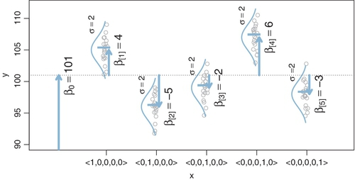
As you may recall from Section 15.2.4.1, we represent the nominal predictor by a vector![]() , where J is the number of categories that the predictor has. When an individual falls in group j of the nominal predictor, this is represented by setting x[j] = 1 and x[i≠j] = 0. The x axis of Figure 19.1 marks the levels of
, where J is the number of categories that the predictor has. When an individual falls in group j of the nominal predictor, this is represented by setting x[j] = 1 and x[i≠j] = 0. The x axis of Figure 19.1 marks the levels of ![]() using this notation. The predicted value, denoted μ, is the overall baseline plus the deflection of a group:
using this notation. The predicted value, denoted μ, is the overall baseline plus the deflection of a group:
where the notation ![]() is called the “dot product” of the vectors. In Equation 19.1, the coefficient β[j] indicates how much the predicted value of y changes when x changes from neutral to category j. The overall baseline is constrained so that the deflections sum to zero across the categories:
is called the “dot product” of the vectors. In Equation 19.1, the coefficient β[j] indicates how much the predicted value of y changes when x changes from neutral to category j. The overall baseline is constrained so that the deflections sum to zero across the categories:
The expression of the model in Equation 19.1 is not complete without the constraint in Equation 19.2.
The sum-to-zero constraint is implemented in the JAGS (or Stan) program in two steps. First, at any point in the MCMC chain, JAGS finds jointly credible values of a baseline and deflections without directly respecting the sum-to-zero constraint. Second, the sum-to-zero constraint is imposed by simply subtracting out the mean of the deflections from the deflections and adding it to the baseline. The algebra is now described formally. Let's denote the unconstrained values of the parameters by α, and denote the sum-to-zero versions by β. At any point in the MCMC chain, the predicted value is

It's easy to show that the β[j] values in Equation 19.4 really do sum to zero:  . A later section shows how Equations 19.3 and 19.4 are implemented in JAGS.
The descriptive model presented in Figure 19.1 is the traditional one used by classical ANOVA (which is described a bit more in the next section). More general models are straight forward to implement in Bayesian software. For example, outliers could be accommodated by using heavy-tailed noise distributions (such as a t distribution) instead of a normal distribution, and different groups could be given different standard deviations. A later section of this chapter explores these generalizations.
19.2 Traditional analysis of variance
The terminology, “analysis of variance,” comes from a decomposition of overall data variance into within-group variance and between-group variance (Fisher, 1925). Algebraically, the sum of squared deviations of the scores from their overall mean equals the sum of squared deviations of the scores from their respective group means plus the sum of squared deviations of the group means from the overall mean. In other words, the total variance can be partitioned into within-group variance plus between-group variance. Because one definition of the word “analysis” is separation into constituent parts, the term ANOVA accurately describes the underlying algebra in the traditional methods. That algebraic relation is not used in the hierarchical Bayesian approach presented here. The Bayesian method can estimate component variances, however. Therefore, the Bayesian approach is not ANOVA, but is analogous to ANOVA.
Traditional ANOVA makes decisions about equality of groups (i.e., null hypotheses) on the basis of p values. As was discussed at length in Chapter 11, and illustrated in Figure 11.1 on p. 299, p values are computed by imaginary sampling from a null hypothesis. In traditional ANOVA, the null hypothesis assumes (i) the data are normally distributed within groups, and (ii) the standard deviation of the data within each group is the same for all groups. The second assumption is sometimes called “homogeneity of variance.” These assumptions are important for mathematical derivation of the sampling distribution. The sample statistic is the ratio of between-group variance to within-group variance, called the F ratio after Ronald Fisher, and therefore the sampling distribution is called the F distribution. For the p value to be accurate, the assumptions of normality and homogeneity of variance should be respected by the data. (Of course, the p value also assumes that the stopping intention is fixed sample size, but that is a separate issue.) These assumptions of normally distributed data with homogeneous variances are entrenched in the traditional approach. That entrenched precedent is why basic models of grouped data make those assumptions, and why the basic models presented in this chapter will also make those assumptions. Fortunately, it is straight forward to relax those assumptions in Bayesian software, where we can use different variance parameters for each group, and use non-normal distributions to describe data within groups, as will be shown later in the chapter.
19.3 Hierarchical bayesian approach
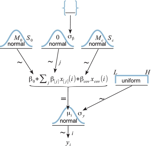
We start with the basic descriptive model that was illustrated in Figure 19.1. Our goal is to estimate its parameters in a Bayesian framework. Therefore, all the parameters need to be given a meaningfully structured prior distribution, which is shown in Figure 19.2. As usual, the hierarchical diagram is scanned from the bottom to the top. At the bottom of Figure 19.2, we see that the data, yi, are distributed normally around the predicted value, μi. The predicted value is specified by Equation 19.1, which is shown in the center of the hierarchical diagram. All the parameters have generic noncommittal prior distributions. Thus, the within-group standard deviation, σy, is given a broad uniform prior distribution (as recommended by Gelman, 2006). The baseline parameter β0, is given a normal prior distribution, made broad on the scale of the data. The group deflection parameters, βj, are given a normal prior distribution that has a mean of zero, because the deflection parameters are supposed to sum to zero. (The sum-to-zero constraint is algebraically imposed later, as described below.)
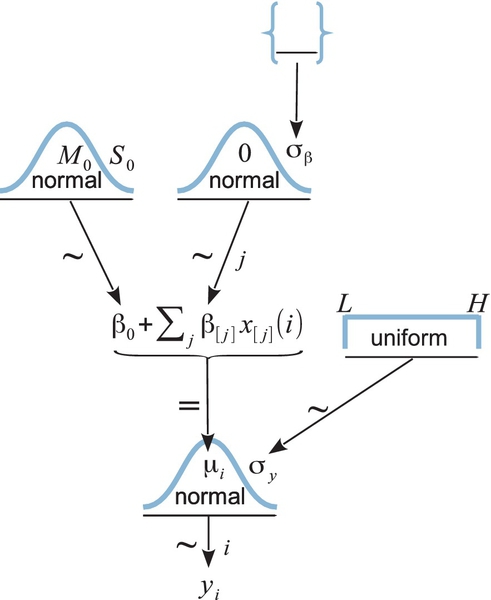
A key novelty of the Bayesian approach is the treatment of σβ, which is the standard deviation of the distribution of deflection parameters. The diagram in Figure 19.2 shows the prior on σβ as a set of empty braces, to suggest that there are options for the prior. One option is that we could just set σβ to a constant. This setting would cause each group deflection to be estimated separately from the other groups, insofar as no group has any influence on the value of σβ. Setting σβ to a large constant results in estimates most analogous to traditional ANOVA.
Instead of fixing σβ at a constant, it can be estimated from the data (Gelman, 2005). If the data suggest that many of the groups have small deflections from baseline, then σβ is estimated to be small. Notice that a small value of σβ imposes strong shrinkage of the estimates of the group deflections. (Shrinkage was explained in Section 9.3 and many examples have been given throughout the book.) When σβ is estimated, the data dictate how much shrinkage to apply to the estimates of the deflection parameters. If many groups are near baseline, then σβ is estimated to be small and the there is strong shrinkage of the group deflections, but if many groups are far from baseline, then σβ is estimated to be large and there is only modest shrinkage of the group deflections.
The form of prior distribution on σβ should reflect genuine prior beliefs and also produce sensible posterior distributions in real applications. Gelman (2006) recommended using a distribution that does not put too much emphasis on values near zero nor on values far from zero, because too much emphasis near zero causes extreme shrinkage, and too much emphasis far from zero causes insufficient shrinkage. He recommended a half-Cauchy or folded-t distribution, which is the positive side of a t distribution. (See Figure 16.4, p. 458, for an illustration of a t distribution.) This distribution puts a finite probability density at zero (unlike a generic gamma (0.001,0.001) distribution on precision), and puts small probability density on large values but with heavy tails that allow for the possibility of large deflections.
In practice, when data sets are small, even a folded-t prior on σβ can yield implosive shrinkage. This can happen because the prior on σβ puts moderately large prior credibility on zero deflections between groups, and the data can be accommodated by setting the group deflections to zero and using a larger value for the within-group noise, σy. (In general, when data sets are small, the prior can have a large influence on the posterior.) There are various reactions we might have to this situation. We could simply accept the implosive shrinkage as the logically correct implication of the assumptions about the prior, if we are committed to the distribution as a firm expression of our prior beliefs. In this case, we need more data to overcome the firm prior beliefs. But if the prior was selected as a default, then the implosive shrinkage could instead be a signal that we should reconsider our assumptions about the prior. For example, the prior distribution on σβ could instead express a belief that deflections of zero are implausible. One way to do that is to use a gamma distribution that has a nonzero mode. This option is implemented in the programs described below.2
A crucial pre-requisite for estimating σβ from all the groups is an assumption that all the groups are representative and informative for the estimate. It only makes sense to influence the estimate of one group with data from the other groups if the groups can be meaningfully described as representative of a shared higher-level distribution. Another way of conceptualizing the hierarchy is that the value of σβ constitutes an informed prior on each group deflection, such that each group deflection has a prior informed by all the other groups. Again, this only makes sense to the extent that the groups can act as prior information for each other. Often this assumption is plausible. For example, in an experiment investigating blood-pressure drugs, all the groups involve blood pressures measured from the same species, and therefore all the groups can reasonably inform an overarching distribution. But if the groups are dominated by a particular subtype, then it might not be appropriate to put them all under a single higher-level distribution. For example, if the experiment involves many different control groups (e.g., various placebos, sham treatments, and no treatments) and only one treatment group, then the presumably small variance between the control groups will make the estimate of σβ small, causing excessive shrinkage of the estimated deflection of the treatment group. One way to address this situation is to use a heavy-tailed distribution to describe the group deflections. The heavy tails allow some deflections to be large. The shape of the higher-level distribution does not change the underlying assumption, however, that all the groups mutually inform each other. If this assumption is not satisfied, it might be best to set σβ to a constant.
19.3.1 Implementation in JAGS
Implementing the model of Figure 19.2 in JAGS is straight forward. Every arrow in the diagram has a corresponding line of code in JAGS. The only truly novel part is implementing the sum-to-zero constraint on the coefficients. We will use the algebraic forms that were presented in Equations 19.3 and 19.4.
In the JAGS model specification below, the noise standard deviation σy is called ySigma, the unconstrained baseline α0 from Equation 19.3 is called a0, and the unconstrained deflection α[j] is called a[j]. The baseline and deflections are subsequently converted to sum-to-zero values called b0 and b[j], respectively. The ![]() value of the ith individual is not coded in JAGS as a vector. Instead, group membership of the ith individual is coded by a simple scalar index called x[i], such that x[i] has value j when the score comes from the jth group. The model specification begins by stating that the individual yi values come from a normal distribution centered at a baseline a0 plus a deflection a[x[i]] for the group, with standard deviation ySigma:
value of the ith individual is not coded in JAGS as a vector. Instead, group membership of the ith individual is coded by a simple scalar index called x[i], such that x[i] has value j when the score comes from the jth group. The model specification begins by stating that the individual yi values come from a normal distribution centered at a baseline a0 plus a deflection a[x[i]] for the group, with standard deviation ySigma:
The code above does not bother to specify mu[i] on a separate line, although it could be written that way and produce the same results.
Next, the priors on ySigma and the baseline a0 are specified. From Figure 19.2, you can see that the prior on ySigma is assumed to be uniform over a range that is wide relative to the scale of the data. We could just ask the user, “What is a typical variance for the type of measurement you are predicting?” and then set the prior wide relative to the answer. Instead, we let the data serve as a proxy and we set the prior wide relative to the variance in the data, called ySD. Analogously, the normal prior for the baseline a0 is centered on the data mean and made very wide relative to the variance of the data. The goal is merely to achieve scale invariance, so that whatever is the measurement scale of the data, the prior will be broad and noncommittal on that scale. Thus,
The model specification continues with the prior on the deflections, a[j]. The standard deviation of the deflections, σβ, is coded as aSigma. The prior on aSigma is a gamma distribution that is broad on the scale of the data, and that has a nonzero mode so that its probability density drops to zero as aSigma approaches zero. Specifically, the shape and rate parameters of the gamma distribution are set so its mode is sd(y)/2 and its standard deviation is 2*sd(y), using the function gammaShRaFromModeSD explained in Section 9.2.2. The resulting shape and rate values are stored in the two-component vector agammaShRa. Thus,
Finally, the sum-to-zero constraint is satisfied by recentering the baseline and deflections according to Equation 19.4. At each step in the MCMC chain, the predicted group means are computed as m[j] <- a0 + a[j]. The baseline is computed as the mean of those group means: b0 <- mean( m[1 : NxLvl] ) where NxLvl is the number of groups (the number of levels of the predictor x). Then the sum-to-zero deflections are computed as the group means minus the new baseline: b[j] <- m[j] - b0. This results in adding mean(a[1 : NxLvl]) to a0 and subtracting mean(a[1 : NxLvl]) from all the a[j], just as in Equation 19.4, but the more elaborate process used here can be generalized to multiple factors (as will be done in the next chapter). Thus, the final section of the model specification is as follows:
The full model is specified in the file Jags-Ymet-Xnom1fac-MnormalHom. R. As explained in Section 8.3 (p. 206), the filename begins with Jags - because it uses JAGS, continues with Ymet- because the predicted variable is metric, then has Xnom1fac-because the predictor is nominal involving a single factor, and finishes with MnormalHom because the model assumes normally distributed data and homogeneous variances. The model is called from the script Jags-Ymet-Xnom1fac-MnormalHom-Example. R.
19.3.2 Example: Sex and death
To illustrate use of the model, we consider the life span of males as a function of the amount of their sexual activity. The data (from Hanley & Shapiro, 1994) are derived from an experiment wherein “sexual activity was manipulated by supplying individual males with receptive virgin females at a rate of one or eight virgins per day. The longevity of these males was recorded and compared with that of two control types. The first control consisted of two sets of individual males kept with newly inseminated females equal in number to the virgin females supplied to the experimental males. The second control was a set of individual males kept with no females. (Partridge & Farquhar, 1981, p. 580)” The researchers were interested in whether male sexual activity reduced life span, as this was already established for females. A deleterious effect of sexual activity would be relatively surprising if found in males because the physiological costs of sexual activity are presumably much lower in males than in females. Oh, I almost forget to mention that the species in question is the fruit fly, Drosophila melanogaster. It is known for this species that newly inseminated females will not remate (for at least two days), and males will not actively court pregnant females. There were 25 male fruit flies in each of the five groups.
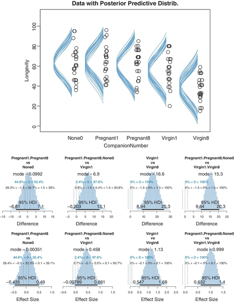
The data are plotted as dots in Figure 19.3. The vertical axis indicates longevity in days. The horizontal axis, labeled “CompanionNumber,” indicates the group. Group None0 indicates the group of males with zero companions. Group Pregnant1 indicates the group of males with one pregnant female. Pregnant8 refers to males accompanied by eight pregnant females. Virgin1 refers to males accompanied by one virgin female, and Virgin8 indicates the males accompanied by eight virgin females. The scatter plot of data suggests that the groups with the receptive females, and hence more sexual activity, had lesser life spans. Our goal is estimate the life spans and the magnitude of differences between groups. (You may recall from Exercise 16.1, p. 473, that sexually deprived male fruit flies are driven to alcohol consumption.)
The five groups in this experiment are all the same type of subjects (male Drosophila) housed in similar apparatus and handled in similar ways except for the specific experimental treatment. Moreover, there was not an overwhelming preponderance of any one type of treatment. Therefore, it is not unreasonable to let the five groups mutually inform each other via the hierarchical model of Figure 19.2, with all groups influencing the estimation of σβ (the standard deviation of the deflections).
It is easy to run the model using the high-level script Jags-Ymet-Xnom1fac-MnormalHom-Example. R. The first step is loading the data file and specifying the column names of the predicted and predictor variables:
After that, the function that calls JAGS is invoked in the usual way:
The argument thinSteps=10 in the function call, above, specifies thinning the chain. As usual, this is merely to keep the saved file size small, but at the cost of somewhat less stability in the posterior estimates. Thinning is not necessary if you don't mind larger files (in which case the number of saved steps should be increased so that the effective sample size is at least 10,000).
The next part of the script is the usual display of MCMC chain diagnostics:
The diagnostic results, not shown here, indicate that the chains are very well behaved, but with some autocorrelation in the standard deviation of the group deflections (i.e., aSigma in the code and σβ in the dependency diagram). Despite the autocorrelation in the high-level variance parameter, the chains are well mixed and the ESS of all the other parameters is at least 10,000.
Figure 19.3 shows posterior predictive distributions superimposed over the data. The curves were created by examining a step in the MCMC chain and plotting normal curves that have the group means and standard deviation at that point in the chain, and repeating for many widely spaced steps in the chain. The smattering of curves looks like a sideways mustache on every group's data. It is important to understand that the bushiness of the mustache represents the uncertainty of the estimate, whereas the width of the mustache represents the value of the standard deviation. For example, a wide mustache that is pencil-thin indicates a large standard deviation that is estimated with high certainty (i.e., small uncertainty). But a narrow mustache that is bushy indicates a small standard deviation that is estimated with poor certainty (i.e., large uncertainty). The bushiness is affected by uncertainty in both the mean and the standard deviation. To get a visual impression of the uncertainty of the mean alone, focus on the spread of the peaks of the curves, not the tails.
Figure 19.3 suggests that the normal distributions with homogeneous variances appear to be reasonable descriptions of the data. There are no dramatic outliers relative to the posterior predicted curves, and the spread of the data within each group appears to be reasonably matched by the width of the posterior normal curves. (Be careful when making visual assessments of homogeneity of variance because the visual spread of the data depends on the sample size; for a reminder see the right panel of Figure 15.9, p. 442.) The range of credible group means, indicated by the peaks of the normal curves, suggests that the group Virgin8 is clearly lower than the others, and the group Virgin1 might be lower than the controls. To find out for sure, we need to examine the differences of group means, which we do in the next section.
19.3.3 Contrasts
For data structured by groups, the researcher is virtually always interested in comparisons between groups or between subsets of groups. In the present application, we might be interested in a large number of paired comparisons. For example, we might be interested in the difference between each of the four treatment groups and the None0 control group. We might be interested in the difference between the Virgin1 group and the Virgin8 group, and the difference between the Pregnant1 group and the Pregnant8 group. We might also be interested in a variety of complex comparisons, which involve differences between averages of sets of groups. For example, we might be interested in the difference between the average of the three control groups (None0, Pregnant1, and Pregnant8) and the average of the two sexually active groups (Virgin1 and Virgin8). Or, we might be interested in the difference between the average of the two unreceptive female groups (Pregnant1 and Pregnant8) and the average of the two sexually active groups. And there are many other comparisons we could make.
It is straight forward to examine the posterior distribution of credible differences. Every step in the MCMC chain provides a combination of group means that are jointly credible, given the data. Therefore, every step in the MCMC chain provides a credible difference between groups, for whatever difference we care to consider. This is the same logic that has been used extensively in this book, for example in Section 9.5.1 regarding baseball batting abilities. Don't forget that the posterior distribution of credible differences cannot be directly discerned from the marginal distributions of individual parameters because the parameters might be correlated, as was explained in Section 12.1.2.1 (p. 340).
To construct the credible differences of group 1 and group 2, at every step in the MCMC chain we compute
In other words, the baseline cancels out of the calculation, and the difference is a sum of weighted group deflections. Notice that the weights sum to zero. To construct the credible differences of the average of groups 1-3 and the average of groups 4-5, at every step in the MCMC chain we compute

Again, the difference is a sum of weighted group deflections. The coefficients on the group deflections have the properties that they sum to zero, with the positive coefficients summing to +1 and the negative coefficients summing to ‒1. Such a combination is called a contrast.3 The differences can also be expressed in terms of effect size, by dividing the difference by σy at each step in the chain.
Contrasts can be specified in the high-level script using meaningful group names instead of arbitrary numerical indices. For example, the Drosophila data file codes the group membership of each subject with a meaningful term. Here are a few lines from the Drosophila data file:
The first line of the data file above specifies the column names. (The “Thorax” column has not yet been used, but will make an appearance later in the chapter.) The important point here is that the CompanionNumber for each subject is indicated by meaningful labels such as Pregnant8, None0, and Pregnant1. We will take advantage of these meaningful labels when specifying contrasts.
In the programs I wrote, a contrast is specified as a list with four components. The first component is a vector of group names whose average constitutes the first element of the comparison. The second component of the list is a vector of group names whose average constitutes the second element of the comparison. The third component of the list is the comparison value, which is typically zero, but could be a nonzero value. The fourth component of the list is a vector specifying the limits of the ROPE, and which could be NULL. Here is an example for the Drosophila data:
The code above defines the variable contrasts as a list of lists. Each component list is a specific contrast that we want to have performed. In the contrasts list above, there are two specific contrasts. The first is a simple paired comparison between Virgin1 and Virgin8. The second is a complex contrast between the average of the three control groups and the average of the two sexually active groups. In both cases, the comparison value is specified as zero (i.e., compVal=0.0)and the ROPE is specified as plus or minus 1.5 days (i.e., ROPE=c (-1.5,1.5)). The list of contrasts can be expanded to include all desired contrasts.
The contrasts list is supplied as an argument to the functions that compute summary statistics and plots of the posterior distribution (plotMCMC and smryMCMC). Some examples of the output of plotMCMC are shown in Figure 19.3. The lower panels show the posterior distribution of the contrasts. The contrasts are displayed on the original scale (days) and on the scale of effect size. Notice that there is a whopping difference of about 15 days (effect size of about 1.0) between the average of the control groups and the average of the sexually active groups, with the 95% HDI falling far outside any reasonable ROPE. On the other hand, the difference between the average of the control groups and the Virgin1 group, while having a mode of about 7 days (effect size just under 0.5), has a posterior distribution that notably overlaps zero and the ROPE.
In traditional ANOVA, analysts often perform a so-called omnibus test that asks whether it is plausible that all the groups are simultaneously exactly equal. I find that the omnibus test is rarely meaningful, however. When the null hypothesis of all-equal groups is rejected, then the analyst is virtually always interested in specific contrasts. Importantly, when the null hypothesis of all-equal groups is not rejected, there can still be specific contrasts that exhibit clear differences (as was shown in Section 12.2.2, p. 348), so again the analyst should examine the specific contrasts of interest. In the hierarchical Bayesian estimation used here, there is no direct equivalent to an omnibus test in ANOVA, and the emphasis is on examining all the meaningful contrasts. An omnibus test can be done with Bayesian model comparison, which is briefly described in Section 20.6.
19.3.4 Multiple comparisons and shrinkage
The previous section suggested that an analyst should investigate all contrasts of interest. This recommendation can be thought to conflict with traditional advice in the context on null hypothesis significance testing, which instead recommends that a minimal number of comparisons should be conducted in order to maximize the power of each test while keeping the overall false alarm rate capped at 5% (or whatever maximum is desired). The issue of multiple comparisons was discussed extensively in Section 11.4 (p. 325), and by specific example in Section 11.1.5 (p. 310). One theme of those sections was that no analysis is immune to false alarms, but a Bayesian analysis eschews the use of p values to control false alarms because p values are based on stopping and testing intentions. Instead, a Bayesian analysis can mitigate false alarms by incorporating prior knowledge into the model. In particular, hierarchical structure (which is an expression of prior knowledge) produces shrinkage of estimates, and shrinkage can help rein in estimates of spurious outlying data. For example, in the posterior distribution from the fruit fly data, the modal values of the posterior group means have a range of 23.2. The sample means of the groups have a range of 26.1. Thus, there is some shrinkage in the estimated means. The amount of shrinkage is dictated only by the data and by the prior structure, not by the intended tests.
Caution: The model can produce implosive shrinkage of group deflections when there are few data points in each group and σβ is estimated (instead of set to a constant). This strong shrinkage occurs because the data can be accommodated by setting all the deflections closer to zero (with small σβ) and with larger noise standard deviation σy. In other words, the model prefers to attribute the overall variance to within-group variability rather than to between-group variability. This preference is not wrong; it is the correct implication of the assumed model structure. If your data involves small sample sizes in each group, and the estimated group means shrink more than seems to be a reasonable description of the data, then it may be a sign that the hierarchical prior is too strong an assumption for the data. Instead, you could set the prior on σβ to a (large) constant. You can try this yourself in Exercise 19.1.
19.3.5 The two-group case
A special case of our current scenario is when there are only two groups. The model of the present section could, in principle, be applied to the two-group case, but the hierarchical structure would do little good because there is virtually no shrinkage when there are so few groups (and the top-level prior on σβ is broad as assumed here). That is why the two-group model in Section 16.3 did not use hierarchical structure, as illustrated in Figure 16.11 (p. 468). That model also used a t distribution to accommodate outliers in the data, and that model allowed for heterogeneous variances across groups. Thus, for two groups, it is more appropriate to use the model of Section 16.3. The hierarchical multi-group model is generalized to accommodate outliers and heterogeneous variances in Section 19.5.
19.4 Including a metric predictor
In Figure 19.3, the data within each group have a large standard deviation. For example, longevities in the Virgin8 group range from 20 to 60 days. With such huge variance of longevities within a group, it is impressive that differences across experimental treatments could be detected at all. For example, the difference between the Virgin1 group and the control groups has an effect size of approximately 0.45 (see Figure 19.3), but the uncertainty in its estimate is large. To improve detectability of differences between groups, it would be useful if some of the within-group variance could be attributed to another measurable influence, so that the effect of the experimental treatment would better stand out.
For instance, suppose that there were some separate measure of how robust a subject is, such that more robust subjects tend to live longer than less robust subjects. We could try to experimentally control the robustness, putting only high-robustness subjects in the experiment. In that way, the variance in longevities, within groups, might be much smaller. Of course, we would also want to run the experiment with medium-robustness subjects and low-robustness subjects. On the other hand, instead of arbitrarily binning the robustness as a nominal predictor, we could simply measure the robustness of randomly included subjects, and use the robustness as a separate metric predictor of longevity. This would allow us to model the distinct influences of robustness and experiment treatment.
An analogous idea was explored in the context of multiple regression in Exercise 18.2 (p. 550). The influence of a primary metric predictor on a predicted variable may appear to be weak because of high residual variance. But a second metric predictor, even if it is uncorrelated with the first predictor, might account for some of the variance in the predicted variable, thereby making the estimate of the slope on the first predictor much more certain.
The additional metric predictor is sometimes called a covariate. In the experimental setting, the focus of interest is usually on the nominal predictor (i.e., the experimental treatments), and the covariate is typically thought of as an ancillary predictor to help isolate the effect of the nominal predictor. But mathematically the nominal and metric predictors have equal status in the model. Let's denote the value of the metric covariate for subject i as xcov(i). Then the expected value of the predicted variable for subject i is
with the usual sum-to-zero constraint on the deflections of the nominal predictor stated in Equation 19.2. In words, Equation 19.5 says that the predicted value for subject i is a baseline plus a deflection due to the group of i plus a shift due to the value of i on the covariate.
It is easy to express the model in a hierarchical diagram, as shown in Figure 19.4. The model has only one change from the diagram in Figure 19.2, namely the inclusion of the covariate in the central formula for μi and a prior distribution on the parameter βcov. The model substructure for the covariate is just like what was used for linear regression in Figures 17.2 (p. 480) and 18.4 (p. 515).
Notice that the baseline in Equation 19.5 is playing double duty. On the one hand, the baseline is supposed to make the nominal deflections sum to zero, so that the baseline represents the overall mean of the predicted data. On the other hand, the baseline is simultaneously acting as the intercept for the linear regression on xcov. It makes sense to set the intercept as the mean of predicted values if the covariate is re-centered at its mean value, which is denoted ![]() . Therefore Equation 19.5 is algebraically reformulated to make the baseline respect those constraints. We start by rewriting Equation 19.5 using unconstrained coefficients denoted as α instead of as β, because we will convert the α expressions into corresponding β values. The first equation below is simply Equation 19.5 with xcov recentered on its mean,
. Therefore Equation 19.5 is algebraically reformulated to make the baseline respect those constraints. We start by rewriting Equation 19.5 using unconstrained coefficients denoted as α instead of as β, because we will convert the α expressions into corresponding β values. The first equation below is simply Equation 19.5 with xcov recentered on its mean, ![]() . The second line below merely algebraically rearranges the terms so that the nominal deflections sum to zero and the constants are combined into the overall baseline:
. The second line below merely algebraically rearranges the terms so that the nominal deflections sum to zero and the constants are combined into the overall baseline:

In the JAGS (or Stan) program for this model, each step in the MCMC chain generates jointly credible values of the α parameters in Equation 19.6, which are then converted to β values that respect the sum-to-zero constraint as indicated by the underbraces in Equation 19.7. The JAGS implementation is in the program Jags-Ymet-Xnom1met1-MnormalHom. R.
19.4.1 Example: Sex, death, and size
We continue with the example from Section 19.3.2, regarding the effect of sexual activity on longevity of male fruit flies. The data were displayed in Figure 19.3 (p. 563) along with posterior predictive distributions. The standard deviation of the noise, σy, which corresponds to the spread (along the y axis) of the normal distributions plotted in Figure 19.3, had a posterior modal value of approximately 14.8 days. This large within-group variance makes it challenging to estimate small between-group differences. For example, the contrast between the sexually deprived males and the Virgin1 group, shown in the second panel of the lower row, suggests about a 7-day difference in longevity, but the uncertainty of the estimate is large, such that the 95% HDI of the difference extends from about zero to almost 14 days.
It turns out that the life span of a fruit fly is highly correlated with its overall size (which asymptotes at maturity). Larger fruit flies live longer. Because fruit flies were randomly assigned to the five treatments, each treatment had a range of fruit flies of different sizes, and therefore much of the within-group variation in longevity could be due to variation is size alone. The researchers measured the size of each fruit fly's thorax, and used the thorax as a covariate in the analysis (Hanley & Shapiro, 1994; Partridge & Farquhar, 1981).
The high-level script Jags-Ymet-Xnom1met1-MnormalHom-Example. R shows how to load the data and run the analysis. The only difference from the previous analysis is that the name of the covariate must be specified, which in this case is “Thorax.” The results of the analysis are shown in Figure 19.5 . The panels in the upper row show the data within each group, plotted as a function of thorax size on the abscissa. Credible posterior descriptions are superimposed on the data. Within the jth group, the superimposed lines show β0+β[j]+βcovxcov for jointly credible values of the parameters at various steps in the MCMC chain. The sideways-plotted normal distributions illustrate the corresponding values of σy for each line.

A key feature to notice is that the within-group noise standard deviation is smaller compared to the previous analysis without the covariate. Specifically, the modal σy is about 10.5 days. The contrast between the sexually deprived males and the Virgin1 group, shown in the second panel of the lower row, now has a 95% HDI that extends from about 4 days to almost 14 days, which clearly excludes a difference of zero and is a more certain estimate than without the covariate. The HDI widths of all the contrasts have gotten smaller by virtue of including the covariate in the analysis.
19.4.2 Analogous to traditional ANCOVA
In traditional frequentist methods, use of the model described above (without hierarchical structure) is called ANCOVA. The best fitting parameter values are derivedas least-squares estimates, and p values are computed from a null hypothesis and fixed-N sampling intention. As mentioned earlier in the context of ANOVA (Section 19.2), Bayesian methods do not partition the least-squares variance to make estimates, and therefore the Bayesian method is analogous to ANCOVA but is not ANCOVA. Frequentist practitioners are urged to test (with p values) whether the assumptions of (a) equal slope in all groups, (b) equal standard deviation in all groups, and (c) normally distributed noise can be rejected. In a Bayesian approach, the descriptive model is generalized to address these concerns, as will be discussed in Section 19.5.
19.4.3 Relation to hierarchical linear regression
The model in this section has similarities to the hierarchical linear regression of Section 17.3. In particular, Figure 17.5 (p. 492) bears a resemblance to Figure 19.5, in that different subsets of data are being fit with lines, and there is hierarchical structure across the subsets of data.
In Figure 17.5, a line was fit to data from each individual, while in Figure 19.5, a line was fit to data from each treatment. Thus, the nominal predictor in Figure 17.5 is individuals, while the nominal predictor in Figure 19.5 is groups. In either case, the nominal predictor affects the intercept term of the predicted value.
The main structural difference between the models is in the slope coefficients on the metric predictor. In the hierarchical linear regression of Section 17.3, each individual is provided with its own distinct slope, but the slopes of different individuals mutually informed each other via a higher-level distribution. In the model of Figure 19.5, all the groups are described using the same slope on the metric predictor. For a more detailed comparison of the model structures, compare the hierarchical diagrams in Figures 17.6 (p. 493) and 19.4 (p. 570).
Conceptually, the main difference between the models is merely the focus of attention. In the hierarchical linear regression model, the focus was on the slope coefficient. In that case, we were trying to estimate the magnitude of the slope, simultaneously for individuals and overall. The intercepts, which describe the levels of the nominal predictor, were of ancillary interest. In the present section, on the other hand, the focus of attention is reversed. We are most interested in the intercepts and their differences between groups, with the slopes on the covariate being of ancillary interest.
19.5 Heterogeneous variances and robustness against outliers
As was mentioned earlier in the chapter, we have assumed normally distributed data within groups, and equal variances across the groups, merely for simplicity and for consistency with traditional ANOVA. We can relax those assumptions in Bayesian software. In this section, we use t distributed noise instead of normal distributions, and we provide every group with its own standard-deviation parameter. Moreover, we put a hierarchical prior on the standard-deviation parameters, so that each group mutually informs the standard deviations of the other groups via the higher-level distribution.
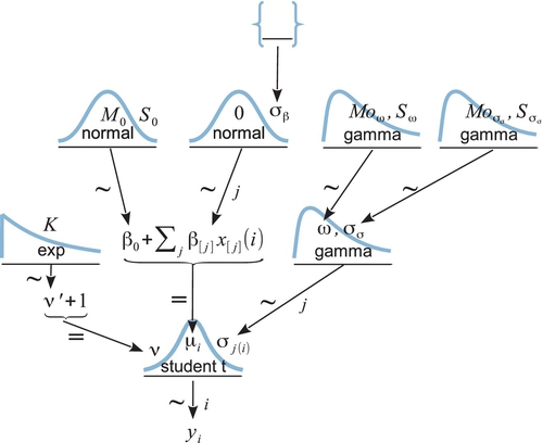
Figure 19.6 shows a hierarchical diagram of the new model. It is merely an extension of the model in Figure 19.2. At the bottom of the diagram, the data yi are described by a t distribution instead of a normal distribution. The t distribution has a normality parameter v annotated on its left, with its prior being the usual prior we have seen previously (e.g., robust estimation of two groups in Figure 16.11, and robust regression in Figure 17.2). The main novelty of Figure 19.6 involves the right-hand side, whichshows the hierarchical prior on the scale parameter of the t distribution. Instead of there being a single σy parameter that applies to all groups, each group has its own scale parameter, σj. The scale parameters of the groups all come from a gamma distribution that has mode ω and standard deviation σσ. The mode and standard deviation of the gamma distribution could be set to constants, so that each group's scale is estimated separately. Instead, we will estimate the modal scale value, and estimate the standard deviation of the scale values. The hierarchical diagram shows that both ω and σσ are given gamma priors that have modes and standard deviations that make them vague on the scale of the data.
The JAGS implementation of the model is a straight-forward extension of the previous model. The only novel part is deciding what should be the constants for the top-level gamma distributions. I have found it convenient to use the same vague prior for all the top-level gamma distributions, but you may, of course, adjust this as appropriate for your application. Recall that the shape and rate values were chosen so that the mode would be sd(y)/2 and the standard deviation would be 2*sd(y):
This choice makes the prior broad on the scale of the data, whatever the scale might happen to be.
In the JAGS model statement, below, you should be able to find corresponding lines of code for each arrow in Figure 19.6. One bit of code that is not in the diagram is the conversion from a gamma distribution's mode and standard deviation to its shape and rate, from Equation 9.8 (p. 238). Hopefully you can recognize that conversion in the following JAGS model specification:
The full program is in the file named Jags-Ymet-Xnom1fac-MrobustHet. R, and the high-level script that calls it is the file named Jags-Ymet-Xnom1fac-MrobustHet-Example. R.
19.5.1 Example: Contrast of means with different variances
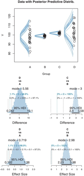
To illustrate the potential usefulness of a model with unequal variances across groups, I have contrived an artificial data set, shown as the dots in Figures 19.7 and 19.8. In this set of data, there are four groups, labeled A, B, C, and D, with means (respectively) of 97, 99, 102, and 104. The standard deviations of the groups are dramatically different, with groups A and D having very large standard deviations relative to groups B and C. The data are randomly sampled from normal distributions.

We first examine the results of applying that model that assumes homogeneous variances (diagrammed in Figure 19.2). The results are shown in Figure 19.7. You can see that the estimated within-group standard deviation seems to be much too big for groupsB and C, but too small for groups A and D. In other words, the estimate of the within-group standard deviation ends up being a compromise between the small-variance and large-variance groups.
An important ramification of the estimates of the within-group variance appears in the contrasts of the means, shown in the bottom of Figure 19.7. The posterior distribution on μD ‒ μA indicates that the difference is clearly greater than zero. On the other hand, the posterior distribution on μC ‒ μB indicates that the difference, while positive, is uncertain enough that zero is within the 95% HDI. But these conclusions seem to conflict with what intuition might suggest from the data themselves. The scatter of data in groups B and C barely overlap, and therefore it seems that the difference should be credibly nonzero. But the scatter of data in groups A and D overlap quite substantially, so it would take a lot of data to convince us that the central tendencies are credibly different.
The problem is that the comparison of μC and μB is using a standard deviation that is too big. The large value ofa widens the normal distribution for describing the data, which lets the μ value slide up and down quite a ways while still keeping the data under the tall part of the normal distribution. Thus, the estimates of μC and μB are “sloppy” and the posterior distribution of their difference is artificially wide. On the other hand, the comparison of and μD and μA is using a standard deviation that is too small. The small value of σ keeps the estimate of μ close to the center of the data. Thus, the estimate of μD ‒ μA is artificially constrained.
When we analyze the data using the model that allows different variances in each group, we get the results shown in Figure 19.8. Notice that the estimated standard deviations of groups B and C are now much smaller than for groups A and D. The description seems far more appropriate than when using equal variances for all the groups.
Importantly, the contrasts of the means in the lower portion of Figure 19.8 are quite different than in Figure 19.7 and make more sense. In Figure 19.8, the posterior estimate of the difference μC ‒ μB is clearly greater than zero, which makes sense because the data of those groups barely overlap. But the posterior estimate of μD ‒ μA, while positive, has a 95% HDI that overlaps a modest ROPE around zero, which also makes sense because the data from the two groups overlap a lot and have only modest sample sizes.
Finally, because each group has its own estimated scale (i.e., σj), we can investigate differences in scales across groups. The difference of scales between groups was implemented by default for the two-group case back in Figure 16.12 (p. 471). The multigroup program does not have contrasts of scales built in, but you can easily create them. For example, at any point after running the mcmcCoda = genMCMC(…) line of the script, you can run the following commands to display the posterior distribution of σ1 ‒ σ2:
In fact, that would make a good exercise; let's call it Exercise 19.3.
19.6 Exercises
Look for more exercises athttps://sites.google.com/site/doingbayesiandataanalysis/
(A) Consider the data file named AnovaShrinkageData.csv, which has columns named Group and Y. How many groups are there? What are the group labels? How many data points per group are there? What are the means of the groups? (Hints: Consider using myDataFrame = read.csv(file=“AnovaShrinkageData. csv”) then aggregate.)
(B) Adapt the high-level script Jags-Ymet-Xnomlfac-MnormalHom-Example. R for reading in AnovaShrinkageData.csv. Set up three contrasts between groups: U vs A, M vs A, and G vs A. Do any of the contrasts suggest a credible non-zero difference between groups? For each of the contrasts, what is the estimated difference between the groups, and what is the actual difference between the sample means of the groups? Include the resulting graphs in your report; see Figure 19.9 for an example. Do any of the graphs look like an inverted funnel, ![]() as was mentioned in Section 18.3?
as was mentioned in Section 18.3?

(C) In the program file Jags-Ymet-Xnomlfac-MnormalHom. R, change the model specification so that σβ is not estimated but is instead fixed at a large value. Specifically, find aSigma and make this change:
Save the program, and then rerun the high-level script with the three contrasts from the previous part. Answer the questions of the previous part, applied to this output. See Figure 19.9 for an example. When you are done with this part, be sure to change the program back to the way it was.
(D) Why are the results of the previous two parts so different? Hint: What is the estimate of aSigma (i.e., σβ) when it is estimated instead of fixed? Discuss why there is so much shrinkage of the group means, for this particular data set, when σβ is estimated.
(A) Run the script Jags-Ymet-Xnom1fac-MnormalHom-Example. R with the Drosophila longevity data, such that the prior distribution is produced. See Section 8.5 for a reminder about how to generate the prior from JAGS. Hint: You only need to comment out a single line in the dataList. Change the fileNameRoot in the script so that you don't overwrite the posterior distribution output.
(B) Continuing with the previous part: Make a fine-bin histogram of the lower part of the prior on σβ (aSigma). Superimpose a curve of the exact gamma distribution using the shape and rate values from the prior specification. Superimpose a vertical line at the mode of the exact gamma distribution. Hints: Make the histogram by usinghist(as.matrix(mcmcCoda)[,”aSigma”] …) with the breaks and xlim set so to reveal the low end of the distributions. Get the shape and rate values of the gamma by using gammaShRaFromModeSD as in the model specification, and then plot the gamma using the lines command. Superimpose a vertical line by using the abline(v=…) command. If you've done it all correctly, the curve for the gamma will closely hug the histogram, and the vertical line will intersect the mode of the curve.
(C) For every parameter, state whether or not the prior is reasonably broad in the vicinity of where the posterior ended up.
(A) Convert the JAGS model in file Jags-Ymet-Xnom1fac-MnormalHom. R to Stan (see Chapter 14). Run it on the Drosophila longevity data and confirm that it produces the same posterior distribution (except for randomness in the MCMC sample).
(B) The JAGS version of the program had fairly low autocorrelation for all parameters except σβ (aSigma). Does Stan show lower autocorrelation for this parameter? To achieve equivalent ESS on the parameters, which of Stan or JAGS takes more real time? (In answering these questions, set thinning to 1 to get a clear comparison.)