
Overview of the Generalized Linear Model
Straight and proportionate, deep in your core
All is orthogonal, ceiling to floor.
But on the outside the vines creep and twist
‘round all the parapets shrouded in mist.1
The previous part of the book explored all the basic concepts of Bayesian analysis applied to a simple likelihood function, namely the Bernoulli distribution. The focus on a simple likelihood function allowed the complex concepts of Bayesian analysis, such as MCMC methods and hierarchical priors, to be developed without interference from additional complications of elaborate likelihood functions with multiple parameters.
In this new part of the book, we apply all the concepts to a more complex but versatile family of models known as the generalized linear model (GLM; McCullagh & Nelder, 1989; Nelder & Wedderburn, 1972). This family of models comprises the traditional “off the shelf” analyses such as t tests, analysis of variance (ANOVA), multiple linear regression, logistic regression, log-linear models, etc. Because we now know from previous chapters the concepts and mechanisms of Bayesian analysis, we can focus on applications ofthis versatile model. The present chapter is important for understanding subsequent chapters because it lays out the framework for all the models in the remainder of the book.
15.1 Types of variables
To understand the GLM and its many specific cases, we must build up a variety of component concepts regarding relationships between variables and how variables are measured in the first place.
15.1.1 Predictor and predicted variables
Suppose we want to predict someone's weight from their height. In this case, weight is the predicted variable and height is the predictor. Or, suppose we want to predict high school grade point average (GPA) from Scholastic Aptitude Test (SAT) score and family income. In this case, GPA is the predicted variable, while SAT score and income are predictor variables. Or, suppose we want to predict the blood pressure of patients who either take drug A, or take drug B, or take a placebo, or merely wait. In this case, the predicted variable is blood pressure, and treatment category is the predictor.
The key mathematical difference between predictor and predicted variables is that the likelihood function expresses the probability of values of the predicted variable as a function ofvalues of the predictor variable. The likelihood function does not describe the probabilities ofvalues of the predictor variable. The value of the predictor variable comes from outside the system being modeled, whereas the value of the predicted variable depends on the value of the predictor variable.
Because the predicted variable depends on the predictor variable, at least mathematically in the likelihood function if not causally in the real world, the predicted variable can also be called the “dependent” variable. The predictor variables are sometimes called “independent” variables. The key conceptual difference between independent and dependent variables is that the value of the dependent variable depends on the value of the independent variable. The term “independent” can be confusing because it can be used strictly or loosely. In experimental settings, the variables that are actually manipulated and set by the experimenter are the independent variables. In this context ofexperimental manipulation, the values of the independent variables truly are (in principle, at least) independent of the values of other variables, because the experimenter has intervened to arbitrarily set the values of the independent variables. But sometimes a non-manipulated variable is also referred to as “independent,” merely as a way to indicate that it is being used as a predictor variable.
Among non-manipulated variables, the roles of predicted and predictor are arbitrary, determined only by the interpretation of the analysis. Consider, for example, people's weights and heights. We could be interested in predicting a person?s weight from his or her height, or we could be interested in predicting a person?s height from his or her weight. Prediction is merely a mathematical dependency, not necessarily a description of underlying causal relationship. Although height and weight tend to co-vary across people, the two variables are not directly causally related. When a person slouches, thereby getting shorter, she does not lose weight. And when a person drinks a glass of water, thereby weighing more, she does not get taller.
Just as “prediction” does not imply causation, “prediction” also does not imply any temporal relation between the variables. For example, we may want to predict a person?s sex, male or female, from his or her height. Because males tend to be taller than females, this prediction can be made with better-than-chance accuracy. But a person?s sex is not caused by his or her height, nor does a person?s sex occur only after their height is measured. Thus, we can “predict” a person?s sex from his or her height, but this does not mean that the person?s sex occurred later in time than his or her height.
In summary, all manipulated independent variables are predictor variables, not predicted. Some dependent variables can take on the role of predictor variables, if desired. All predicted variables are dependent variables. The likelihood function specifies the probability of values of the predicted variables as a function of the values of the predictor variables.
Why we care: We care about these distinctions between predicted and predictor variables because the likelihood function is a mathematical description of the dependency of the predicted variable on the predictor variable. The first thing we have to do in statistical inference is identify what variables we are interested in predicting, on the basis of what predictors. As you should recall from Section 2.3, p. 25, the first step of Bayesian data analysis is to identify the data relevant to the analysis, and which variables are predictors and which variable is predicted.
15.1.2 Scale types: metric, ordinal, nominal, and count
Items can be measured on different scales. For example, the participants in a foot race can be measured either by the time they took to run the race, or by their placing in the race (first, second, third, etc.), or by the name of the team they represent. These three measurements are examples of metric, ordinal, and nominal scales, respectively (Stevens, 1946).
Examples of metric scales include response time (i.e., latency or duration), temperature, height, and weight. Those are actually cases of a specific type of metric scale called a ratio scale, because they have a natural zero point on the scale. The zero point on the scale corresponds to there being a complete absence of the stuff being measured. For example, when the duration is zero, there has been no time elapsed, and when the weight is zero, there is no downward force. Because these scales have a natural zero point, it is meaningful to talk about ratios of amounts being measured, and that is why they are called ratio scales. For example, it is meaningful to say that taking 2 min to solve a problem is twice as long as taking 1 min to solve the problem. On the other hand, the scale of historical time has no known absolute zero. We cannot say, for example, that there is twice as much time in January 2nd as there is time in January 1st. We can refer to the duration since some arbitrary reference point, but we cannot talk about the absolute amount of time in any given moment. Scales that have no natural zero are called interval scales because all we know about them is the amount of stuff in an interval on the scale, not the amount of stuff at a point on the scale. Despite the conceptual difference between ratio and interval scales, I will lump them together into the category of metric scales.
A special case of metric-scaled data is count data, also called frequency data. For example, the number of cars that pass through an intersection during an hour is a count. The number of poll respondents who say they belong to a particular political party is a count. Count data can only have values that are nonnegative integers. Distances between counts have meaning, and therefore the data are metric, but because the data cannot be negative and are not continuous, they are treated with different mathematical forms than continuous, real-valued metric data.
Examples of ordinal scales include placing in a race, or rating of degree of agreement. When we are told that, in a race, Jane came in first, Jill came in second, and Jasmine came in third, we only know the order. We do not know whether Jane beat Jill by a nose or by a mile. There is no distance or metric information in an ordinal scale. As another example, many polls have ordinal response scales: Indicate how much you agree with this statement: “Bayesian statistical inference is better than null hypothesis significance testing,” with 5 = strongly agree, 4 = mildly agree, 3 = neither agree nor disagree, 2 = mildly disagree, and 1 = strongly disagree. Notice that there is no metric information in the response scale, because we cannot say the difference between ratings of 5 and 4 is the same amount of difference as between ratings of 4 and 3.
Examples of nominal, a.k.a. categorical, scales include political party affiliation, the face of a rolled die, and the result of a flipped coin. For nominal scales, there is neither distance between categories nor order between categories. For example, suppose we measure the political party affiliation of a person. The categories of the scale might be Green, Democrat, Republican, Libertarian, and Other (in the United States, with different parties in different countries). While some political theories might suggest that the parties fall on an underlying liberal-conservative scale, there is no such scale in the actual categorical values themselves. In the actual categorical labels there is neither distance nor ordering. As another example of values on a nominal scale, consider eye color and hair color, as in Table 4.1, p. 90. Both eye color and hair color are nominal variables because they have neither distance between levels nor ordering of levels. The cells of Table 4.1 show count data that may be predicted from the nominal color predictors, as will be explored in Chapter 24.
In summary, if two items have different nominal values, all we know is that the two items are different (and what categories they are in). On the other hand, if two items have different ordinal values, we know that the two items are different and we know which one is “larger” than the other, but not how much larger. If two items have different metric values, then we know that they are different, which one is larger, and how much larger.
Why we care: We care about the scale type because the likelihood function must specify a probability distribution on the appropriate scale. If the scale has two nominal values, then a Bernoulli likelihood function may be appropriate. If the scale is metric, then a normal distribution may be appropriate as a probability distribution to describe the data. Whenever we are choosing a model for data, we must answer the question, What kind of scale are we dealing with? As you should recall from Section 2.3, p. 25, the first step of Bayesian data analysis includes identifying the measurement scales of the predictor and predicted variables.
In the following sections, we will first consider the case of a metric-predicted variable with metric predictors. In that context of all metric variables, we will develop the concepts of linear functions and interactions. Once those concepts are established for metric predictors, the notions will be extended to nominal predictors.
15.2 Linear combination of predictors
The core of the GLM is expressing the combined influence of predictors as their weighted sum. The following sections build this idea by scaffolding from the simplest intuitive cases.
15.2.1 Linear function of a single metric predictor
Suppose we have identified one variable to be predicted, which we?ll call y, and one variable to be the predictor, which we?ll call x. Suppose we have determined that both variables are metric. The next issue we need to address is how to model a relationship between x and y. This is now Step 2 of Bayesian data analysis from Section 2.3, p. 25. There are many possible dependencies of y on x, and the particular form of the dependency is determined by the specific meanings and nature of the variables. But in general, across all possible domains, what is the most basic or simplistic dependency of y on x that we mightconsider? The usual answer to this question is: a linear relationship. A linear function is the generic, “vanilla,” off-the-shelf dependency that is used in statistical models.
Linear functions preserve proportionality (relative to an appropriate baseline). If you double the input, then you double the output. If the cost of a candy bar is a linear function of its weight, then when the weight is reduced 10%, the cost should be reduced 10%. If automobile speed is a linear function of fuel injection to the engine, then when you press the gas pedal 20% further, the car should go 20% faster. Nonlinear functions do not preserve proportionality. For example, in actuality, car speed is not a linear function of the amount of fuel consumed. At higher and higher speeds, it takes proportionally more and more gas to make the car go faster. Despite the fact that many real-world dependencies are nonlinear, most are at least approximately linear over moderate ranges of the variables. For example, If you have twice the wall area, it takes approximately twice the amount of paint. It is also the case that linear relationships are intuitively prominent (Brehmer, 1974; P.J. Hoffman, Earle, & Slovic, 1981; Kalish, Griffiths, & Lewandowsky, 2007). Linear relationships are the easiest to think about: Turn the steering wheel twice as far, and we believe that the car should turn twice as sharp. Turn the volume knob 50% higher, and we believe that the loudness should increase 50%.
The general mathematical form for a linear function of a single variable is
When values of x and y that satisfy Equation 15.1 are plotted, they form a line. Examples are shown in Figure 15.1. The value of parameter β0 is called the y-intercept because it is where the line intersects the y-axis when x = 0. The left panel of Figure 15.1 shows two lines with different y-intercepts. The value of parameter β1 is called the slope because it indicates how much y increases when x increase by 1. The right panel of Figure 15.1 shows two lines with the same intercept but different slopes.

In strict mathematical terminology, the type of transformation in Equation 15.1 is called affine. When β ≠ 0, the transformation does not preserve proportionality. For example, consider y = 10 + 2x. When x is doubled from x = 1 to x = 2, y increases from y = 12 to y = 14, which is not doubling y. Nevertheless, the rate of increase in y is the same for all values of x: Whenever x increases by 1, y increases by β1. Moreover, Equation 15.1 can have either y or x shifted so that proportionality is achieved. If y is simply shifted by β0 and the shifted value is called y∗, then proportionality is achieved: y∗ = y—β0 = β1x. Or, if x is shifted by — β0/β1 and the shifted value is called x∗, then proportionality is achieved: y=β1(x-β0/β1)=β1x∗. This form of the equation is called x-intercept form or x-threshold form, because —β0/β1 is where the line crosses the x-axis, and is the threshold between negative and positive values of y.
Summary of why we care. The likelihood function includes the form of the dependency of y on x. When y and x are metric variables, the simplest form of dependency, both mathematically and intuitively, is one that preserves proportionality. The mathematical expression of this relation is a so-called linear function. The usual mathematical expression of a line is the y-intercept form, but sometimes a more intuitive expression is the x threshold form. Linear functions form the core of the GLM.
15.2.2 Additive combination of metric predictors
If we have more than one predictor variable, what function should we use to combine the influences of all the predictor variables? If we want the combination to be linear in each of the predictor variables, then there is just one answer: Addition. In other words, if we want an increase in one predictor variable to predict the same increase in the predicted variable for any value of the other predictor variables, then the predictions of the individual predictor variables must be added.
In general, a linear combination of K predictor variables has the form

Figure 15.2 shows examples of linear functions of two variables, x1 and x2. The graphs show y plotted only over a the domain with 0 ≤ x1 ≤ 10 and x2 ≤ 10. It is important to realize that the plane extends from minus to plus infinity, and the graphs only show a small region. Notice in the upper left panel, where y = 0 + 1x1 + 0x2,the plane tilts upward in the x1 direction, but the plane is horizontal in the x2 direction. For example, when x1= 10 then y = 10 regardless of the value of x2 The opposite is true in the upper right panel, where y = 0+x1 + 2x2. In this case, the plane tilts upward in the x2 direction, but the plane is horizontal in the x1 direction. The lower left panel shows the two influences added: y = 0+x1 + 2x2. Notice that the slope in the x2 direction is steeper than in the x1 direction. Most importantly, notice that the slope in the x2 direction is the same at any specific value of x1. For example, when x1 is fixed at 0, then y rises from y = 0to y = 20 when x2 goes from x2 = 0to x2 = 10. When x1 is fixed at 10, then y again rises 20 units, from y = 10 to y = 30.

Summary of section: When the influence of every individual predictor is unchanged by changing the values of other predictors, then the influences are additive. The combined influence of two or more predictors can be additive even if the individual influences are nonlinear. But if the individual influences are linear, and the combined influence is additive, then the overall combined influence is also linear. The formula of Equation 15.2 is one expression of a linear model, which forms the core of the GLM.
15.2.3 Nonadditive interaction of metric predictors
The combined influence of two predictors does not have to be additive. Consider, for example, a person?s self-rating of happiness, predicted from his or her overall health and annual income. It?s likely that if a person?s health is very poor, then the person is not happy, regardless of his or her income. And if the person has zero income, then the person is probably not happy, regardless of his or her health. But if the person is both healthy and rich, then the person has a higher probability of being happy (despite celebrated counter-examples in the popular media).
A graph of this sort of nonadditive interaction between predictors appears in the upper left panel of Figure 15.3. The vertical axis, labeled y, is happiness. The horizontal axes, x1 and x2, are health and income. Notice that if either x1= 0 orx2= 0, then y= 0. But if both x1 > 0and x2x2 0, then y> 0. The specific form of interaction plotted here is multiplicative: y = 0+0x1+0x2+0.2x1x2. For comparison, the upper right panel of Figure 15.3 shows a non-interactive (i.e., additive) combination of x1 and x2. Notice that the graph of the interaction has a twist or curvature in it, but the graph of the additive combination is flat.

The lower left panel of Figure 15.3 shows a multiplicative interaction in which the individual predictors increase the outcome, but the combined variables decrease the outcome. A real-world example of this occurs with some drugs: Individually, each of two drugs might improve symptoms, but when taken together, the two drugs might interact and cause a decline in health. As another example, consider lighter-than-air travel in the form of ballooning. The levity of a balloon can be increased by fire, as in hot air balloons. And the levity of a balloon can be increased by hydrogen, as in many early twentieth century blimps and dirigibles. But the levity of a balloon is dramatically decreased by the combination of fire and hydrogen.
The lower right panel of Figure 15.3 shows a multiplicative interaction in which the direction of influence of one variable depends on the magnitude of the other variable. Notice that when x2=0, then an increase in the x1 variable leads to a decline in y. But whenx2, then an increase in the x2 variable leads to an increase in y. Again, the graph of the interaction shows a twist or curvature; the surface is not flat.
There is a subtlety in the use of the term “linear” that can sometimes cause confusion in this context. The interactions shown in Figure 15.3 are not linear on the two predictors x1 and x2. But if the product of the two predictors, x1x2, is thought of as a third predictor, then the model is linear on the three predictors, because the predicted value of y is a weighted additive combination of the three predictors. This reconceptualization can be useful for implementing nonlinear interactions in software for linear models, but we will not be making that semantic leap to a third predictor, and instead we will think of a nonadditive combination of two predictors.
A nonadditive interaction of predictors does not have to be multiplicative. Other types of interaction are possible. The type of interaction is motivated by idiosyncratic theories for different variables in different application domains. Consider, for example, predicting the magnitude of gravitational force between two objects from three predictor variables: the mass of object one, the mass of object two, and the distance between the objects. The force is proportional to the multiplicative product of the two masses divided by the squared distance between them.
15.2.4 Nominal predictors
15.2.4.1 Linear model for a single nominal predictor
The previous sections assumed that the predictor was metric. But what if the predictor is nominal, such as political party affiliation or sex? A convenient formulation has each value of the nominal predictor generate a particular deflection of y away from its baseline level. For example, consider predicting height from sex (male or female2). We can consider the overall average height across both sexes as the baseline height. When an individual has the value “male,” that adds an upward deflection to the predicted height. When an individual has the value “female,” that adds a downward deflection to the predicted height.
Expressing that idea in mathematical notation can get a little awkward. First consider the nominal predictor. We can?t represent it appropriately as a single scalar value, such as 1 through 5, because that would suggest that level 1 is closer to level 2 than it is to level 5, which is not true of nominal values. Therefore, instead of representing the value of the nominal predictor by a single scalar value x, we will represent the nominal predictor by avector ![]() , where J is the number of categories that the predictor has. As you may have just noticed, I will use a subscript in square brackets to indicate a particular element of the vector, by analogy to indices in R. Thus, the first component of
, where J is the number of categories that the predictor has. As you may have just noticed, I will use a subscript in square brackets to indicate a particular element of the vector, by analogy to indices in R. Thus, the first component of ![]() is denoted x[1] and the jth component is denoted x[j] When an individual has level j of the nominal predictor, this is represented by setting x[j]=1 and x[i≠j] =0. For example, suppose x is sex, with level 1 being male and level 2 being female. Then male is represented as
is denoted x[1] and the jth component is denoted x[j] When an individual has level j of the nominal predictor, this is represented by setting x[j]=1 and x[i≠j] =0. For example, suppose x is sex, with level 1 being male and level 2 being female. Then male is represented as ![]() and female is represented as
and female is represented as ![]() . As another example, suppose that the predictor is political party affiliation, with Green as level 1, Democrat as level 2, Republican as level 3, Libertarian as level 4, and Other as level 5. Then Democrat is represented as
. As another example, suppose that the predictor is political party affiliation, with Green as level 1, Democrat as level 2, Republican as level 3, Libertarian as level 4, and Other as level 5. Then Democrat is represented as ![]() and Libertarian is represented as
and Libertarian is represented as ![]()
Now that we have a formal representation for the nominal predictor variable, we can create a formal representation for the generic model of how the predictor influences the predicted variable. As mentioned above, the idea is that there is a baseline level of the predicted variable, and each category of the predictor indicates a deflection above or below that baseline level. We will denote the baseline value of the prediction as β0. The deflection for the jth level of the predictor is denoted β[j]. Then the predicted value is
where the notation ![]() is sometimes called the “dot product” of the vectors.
is sometimes called the “dot product” of the vectors.
Notice that Equation 15.3 has a form similar to the basic linear form of Equation 15.1. The conceptual analogy is this: In Equation 15.1 for a metric predictor, the coefficient β1 indicates how much y changes when x changes from 0 to 1. In Equation 15.3 for a nominal predictor, the coefficient β[j] indicates how much y changes when x changes from neutral to category j.
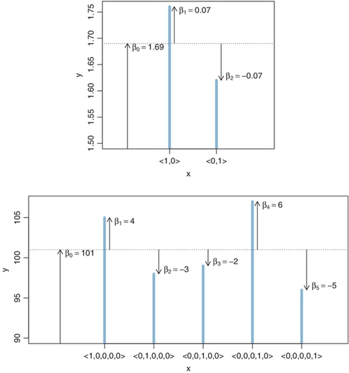
There is one more consideration when expressing the influence of a nominal predictor as in Equation 15.3: How should the baseline value be set? Consider, for example, predicting height from sex. We could set the baseline height to be zero. Then the deflection from baseline for male might be 1.76 m, and the deflection from baseline for female might be 1.62 m. On the other hand, we could set the baseline height to be 1.69 m. Then the deflection from baseline for male would be +0.07 m, and the deflection from baseline for female would be −0.07 m. The second way of setting the baseline is a typical form in generic statistical modeling. In other words, the baseline is constrained so that the deflections sum to zero across the categories:
The expression of the model in Equation 15.3 is not complete without the constraint in 15.4. Figure 15.4 shows examples of a nominal predictor expressed in terms of Equations 15.3 and 15.4. Notice that the deflections from baseline sum to zero, as demanded by the constraint in Equation 15.4.
15.2.4.2 Additive combination of nominal predictors
Suppose we have two (or more) nominal predictors of a metric value. For example, we might be interested in predicting income as a function of political party affiliation and sex. Figure 15.4 showed examples of each of those predictors individually (for different predicted variables). Now we consider the joint influence of those predictors. If the two influences are additive, then the model from Equation 15.3 becomes

with the constraints
The left panel of Figure 15.5 shows an example of two nominal predictors that have additive effects on the predicted variable. In this case, the overall baseline is y = 5. When x1 = (1,0), there is a deflection in y of −1, and when x1 = (0,1), there is a deflection in y of +1. These deflections by x1 are the same at every level of x2 The deflections for the three levels of x2 are +3, −2, and −1. These deflections by x2 are the same at all levels of x1. Formally, the left panel of Figure 15.5 is expressed mathematically by the additive combination:
For example, consider ![]() and
and ![]() . According to Equation 15.7, the value of the predicted variable is y = 5 + 〈 —1,1 〈0,1〉 + 〈3, —2, —1〉-〈0, 0,1〉 = 5 + 1 1 = 5, which does indeed match the corresponding bar in the left panel of Figure 15.5.
. According to Equation 15.7, the value of the predicted variable is y = 5 + 〈 —1,1 〈0,1〉 + 〈3, —2, —1〉-〈0, 0,1〉 = 5 + 1 1 = 5, which does indeed match the corresponding bar in the left panel of Figure 15.5.

15.2.4.3 Nonadditive interaction of nominal predictors
In many applications, an additive model is not adequate for describing the combined influence of two predictors. For example, consider predicting annual income from political party affiliation and sex (in the contemporary United States). Men, on average, have a higher income than women. Republicans, on average, have a higher income than Democrats. But it may be that the influences of sex and political party combine nonadditively: Perhaps people who are both Republican and male have a higher average income than would be predicted by merely adding the average income boosts for being Republican and for being male. (This nonadditive interaction is not claimed to be true; it is being used only as a hypothetical example.)
We need new notation to formalize the nonadditive influence of a combination of nominal values. Just as ![]() refers to the value of predictor 1, and
refers to the value of predictor 1, and ![]() refers to the value of predictor 2, the notation
refers to the value of predictor 2, the notation ![]() will refer to a particular combination of values of predictors 1 and 2. If there are
will refer to a particular combination of values of predictors 1 and 2. If there are ![]() levels of predictor 1 and
levels of predictor 1 and ![]() levels of predictor 2, then there are
levels of predictor 2, then there are ![]() combinations of the two predictors. To indicate a particular combination of levels from predictors 1 and 2, the corresponding component of
combinations of the two predictors. To indicate a particular combination of levels from predictors 1 and 2, the corresponding component of ![]() is set to 1 while all other components are set to 0. A nonadditive interaction of predictors is formally represented by including a term for the influence of combinations of predictors, beyond the additive influences, as follows:
is set to 1 while all other components are set to 0. A nonadditive interaction of predictors is formally represented by including a term for the influence of combinations of predictors, beyond the additive influences, as follows: ![]() .
.
The right panel of Figure 15.5 shows a graphical example of two nominal predictors that have interactive (i.e., nonadditive) effects on the predicted variable. Notice, in the left pair of bars (x2 ={1,0, 0)), that a change from x1 = 〈1,0〉 to x1 = 〈0,1〉 produces an increase of +4 in y, from y = 6 to y = 10. But for the middle pair of bars (x2 = 〈0, 1, 0〉), a change from x1 = 〈1, 0〉 to x1 = 〈0, 1〉 produces a change of −2 in y, from y = 4 down to y = 2. Thus, the influence of x1 is not the same at all levels of x2. Formally, the right panel of Figure 15.5 is expressed mathematically by the combination:
The interaction coefficients, ![]() , have been displayed in two rows like a matrix to make it easier to understand which component corresponds to which combination of levels The two rows correspond to the two levels of
, have been displayed in two rows like a matrix to make it easier to understand which component corresponds to which combination of levels The two rows correspond to the two levels of ![]() and the three columns correspond to the three levels of
and the three columns correspond to the three levels of ![]() For example, consider
For example, consider ![]() and
and ![]() . According to Equation 15.8, the value of the predicted variable is
. According to Equation 15.8, the value of the predicted variable is

which does indeed match the corresponding bar in the right panel of Figure 15.5.
An interesting aspect of the pattern in the right panel of Figure 15.5 is that the average influences of x1 and x2 are the same as in the left panel. Overall, on average, going from x1 = 〈1, 0〉 to x1 = 〈0, 1〉 produces a change of +2 in y, in both the left and right panels. And overall, on average, for both panels it is the case that x2 = 〈1, 0, 0〉 is +3 above baseline, x2 =〈0,1,0〉 is −2 below baseline, and x2 =〈0, 0,1〉 is −1 below baseline. The only difference between the two panels is that the combined influence of the two predictors equals the sum of the individual influences in the left panel, but the combined influence of the two predictors does not equal the sum of the individual influences in the right panel. This appears explicitly in Equations 15.7 and 15.8: The only difference between them is the interaction coefficients, which are (tacitly) zero in Equation 15.7.
In general, the expression that includes an interaction term can be written as

with the constraints

Notice that these constraints were satisfied in the example of Equation 15.8. In particular, within every row and every column of the matrix representation of ![]() , the coefficients summed to zero.
, the coefficients summed to zero.
The notation used here is a bit unwieldy, so do not fret if is not clear to you yet. That?s my fault, not yours, because I?m only presenting an overview at this point. When we implement these ideas in Chapter 20 there will be more examples and different notation for computer programs. The main point to understand now is that the term “interaction” refers to a nonadditive influence of the predictors on the predicted, regardless of whether the predictors are measured on a nominal scale or a metric scale.
Summary: We have now seen how predictors of different scale types are weighted and added together to form an underlying trend for the predicted variable. Table 15.1 shows a summary of the cases we have covered. Each column of Table 15.1 corresponds to a type of predictor, and the cells of the table show the mathematical form of the linear combination. As a general notation to refer to these linear functions of predictors, I will use the expression lin(x). For example, when there is a single metric predictor, lin(x) = β0 + β1x. All of the cells in Table 15.1 show forms of lin(x). Even if there are multiple predictors, the notation lin(x) refers to a linear combination of all of them.
Table 15.1
For the generalized linear model: typical linear functions lin(x) of the predictor variables x, for various scale types of x
| Scale type of predictor x | |||||
| Metric | Nominal | ||||
| Single group | Two groups | Single predictor | Multiple predictors | Single factor | Multiple factor |
| β0 | β0+β1x |  | |||

The value lin(x) is mapped to the predicted data by functions shown in Table 15.2.
Table 15.1 also indicates a few special cases and generalizations not previously mentioned. In the left columns of the table, the special cases of one or two groups are shown. When there is a single group, then the predictor x is merely a single value, namely, an indicator of being in the group. It does not matter if we think of this single value as nominal or ordinal or metric because all we are describing with the linear core is the central tendency of the group, denoted ¡0. When there are two groups, the predictor x is a nominal indicator of group membership. We could subsume the two-group case under the column for a nominal, single-factor predictor (as was shown, for example, in the top panel of Figure 15.4), but the two-group case is encountered so often that we give it a column of its own. Finally, in the columns of Table 15.1 for multiple predictors, the formulas for lin(x) include optional terms for higher order interactions. Just as any two predictors may have combined effects that are not captured by merely summing their separate influences, there may be effects of multiple predictors that are not captured by two-way combinations. In other words, the magnitudes of the two-way interactions might depend on the levels of other predictors. Higher order interactions are routinely incorporated into models of nominal predictors, but relatively rarely used in models of metric predictors.
15.3 Linking from combined predictors to noisy predicted data
15.3.1 From predictors to predicted central tendency
After the predictor variables are combined, they need to be mapped to the predicted variable. This mathematical mapping is called the (inverse) link function, and is denoted by f() in the following equation:
Until now, we have been assuming that the link function is merely the identity function, f(lin(x)) = lin(x). For example, in Equation 15.9, y equals the linear combination of the predictors; there is no transformation of the linear combination before mapping the result to y.
Before describing different link functions, it is important to make some clarifications ofterminology and corresponding concepts. First, the function f() in Equation 15.11 is called the inverse link function, because the link function is traditionally thought of as transforming the value y into a form that can be linked to the linear model. That is, the link function goes from y to the predictors, not from the predictors to y. Imay occasionally abuse convention and refer to either f() or f−1() as “the” link function, and rely on context to disambiguate which direction of linkage is intended. The reason for this terminological sadism is that the arrows in hierarchical diagrams of Bayesian models will flow from the linear combination toward the data, and therefore it is natural for the functions to map toward the predicted values, as in Equation 15.11. But repeatedly referring to this function as the “inverse” link would strain my patience and violate my aesthetic sensibilities. Second, the value y that results from the link function f(lin(x)) is not a data value per se. Instead,f(lin(x)) is the value of a parameter that expresses a central tendency of the data, usually their mean. Therefore the function f() in Equation 15.11 is sometimes called the mean function (instead of the inverse link function), and is written μ = f() instead of y = f(). I will use this notation temporarily for some summary tables below, but then abandon it because f() does not always refer to the mean of the predicted data.
There are situations in which a non-identity link function is appropriate. Consider, for example, predicting response time as a function of amount of caffeine consumed. Response time decreases as caffeine dosage increases (e.g., Smit & Rogers, 2000, Fig. 1; although most of the decrease is produced by even a small dose). Therefore a linear prediction of RT (y)from dosage(x) would have a negative slope. This negative slope on a linear function implies that for a very large dosage of caffeine, response time would become negative, which is impossible unless caffeine causes precognition (i.e., foreseeing events before they occur). Therefore a linear function cannot be used for extrapolation to large doses, and we might instead want to use a link function that asymptotes above zero, such as an exponential function with y = exp + (β0+β1x). In the next sections we will consider some frequently used link functions.
15.3.1.1 The logistic function
A frequently used link function is the logistic:
Notice the negative sign in front of the x. The value y of the logistic function ranges between 0 and 1. The logistic is nearly 0 when x is large negative, and is nearly 1 when x is large positive. In our applications, x is a linear combinations of predictors. For a single metric predictor, the logistic can be written:
The logistic function is often most conveniently parameterized in a form that shows the gain γ (Greek letter gamma) and threshold θ:
Examples of Equation 15.14 are shown in Figure 15.6. Notice that the threshold is the point on the x-axisfor which y = 0.5. The gain indicates how steeply the logistic rises through that point.

Figure 15.7 shows examples of a logistic of two predictor variables. Above each panel is the equation for the corresponding graph. The equations are parameterized in normalized-threshold form: ![]() , with
, with ![]() . Notice, in particular, that the coefficients of x1 and x2 in the plotted equations do indeed have Euclidean length of 1.0. For example, in the upper right panel, (0.712 + 0.712)1/2 = 1.0, except for rounding error. If you start with the linear part parameterized as
. Notice, in particular, that the coefficients of x1 and x2 in the plotted equations do indeed have Euclidean length of 1.0. For example, in the upper right panel, (0.712 + 0.712)1/2 = 1.0, except for rounding error. If you start with the linear part parameterized as ![]() you can convert to the equivalent normalized-threshold form as follows: Let
you can convert to the equivalent normalized-threshold form as follows: Let ![]() ,and
,and ![]() .
.

The coefficients of the x variables determine the orientation of the logistical “cliff.” For example, compare the two top panels in Figure 15.7, which differ only in the coefficients, not in gain or threshold. In the top left panel, the coefficients are W1 = 0 and W2 = 1, and the cliff rises in the x2 direction. In the top right panel, the coefficients are W1 = 0.71 and W2 = 0.71, and the cliff rises in the positive diagonal direction.
The threshold determines the position of the logistical cliff. In other words, the threshold determines the x values for which y = 0.5. For example, compare the two left panels of Figure 15.7. The coefficients are the same, but the thresholds (and gains) are different. In the upper left panel, the threshold is zero, and therefore the mid-level of the cliff is over x2 = 0. In the lower left panel, the threshold is −3, and therefore the mid-level of the cliff is over x2 = −3.
The gain determines the steepness of the logistical cliff. Again compare the two left panels of Figure 15.7. The gain of the upper left is 1, whereas the gain of the lower left is 2.
Terminology: The logit function. The inverse of the logistic function is called the logit function. For 0 < p < 1, logit(p) = log (p/(1 − p)). It is easy to show(try it!) that logit(logistic(x)) = x, which is to say that the logit is indeed the inverse of the logistic. Some authors, and programmers, prefer to express the connection between predictors and predicted in the opposite direction, by first transforming the predicted variable to match the linear model. In other words, you may see the link expressed either of these ways:
The two expressions achieve the same result, mathematically. The difference between them is merely a matter of emphasis. In the first expression, the combination of predictors is transformed so it maps onto y. In the second expression, y is transformed onto a new scale, and that transformed value is modeled as a linear combination of predictors. I find that the logistic formulation is usually more intuitive than the logit formulation, but we will see in Chapter 21 that the logit formulation will be useful for interpreting the β coefficients.
15.3.1.2 The cumulative normal function
Another frequently used link function is the cumulative normal distribution. It is qualitatively very similar to the logistic function. Modelers will use the logistic or the cumulative normal depending on mathematical convenience or ease of interpretation. For example, when we consider ordinal predicted variables (in Chapter 23), it will be natural to model the responses in terms of a continuous underlying variable that has normally distributed variability, which leads to using the cumulative normal as a model of response probabilities.
The cumulative normal is denoted Φ(x; μ, σ, where x is a real number and where μ and σ are parameter values, called the mean and standard deviation of the normal distribution. The parameter μ governs the point at which the cumulative normal, Φ(x), equals 0.5. In other words, μ plays the same role as the threshold in the logistic. The parameter σ governs the steepness of the cumulative normal function at x = μ, but inversely, such that a smaller value of σ corresponds to a steeper cumulative normal. A graph of a cumulative standardized normal appears in Figure 15.8.

Terminology: The inverse of the cumulative normal is called the probit function. (“Probit” stands for “probability unit”; Bliss, 1934). The probit function maps a value p,for ![]() , onto the infinite real line, and a graph of the probit function looks very much like the logit function. You may see the link expressed either of these ways:
, onto the infinite real line, and a graph of the probit function looks very much like the logit function. You may see the link expressed either of these ways:
Traditionally, the transformation of y (in this case, the probit function) is called the link function, and the transformation of the linear combination of x (in this case, the Φ function) is called the inverse link function. As mentioned before, I abuse the traditional terminology and call either one a link function, relying on context to disambiguate. In later applications, we will be using the $ function, not the probit.
15.3.2 From predicted central tendency to noisy data
In the real world, there is always variation in y that we cannot predict from x. This unpredictable “noise” in y might be deterministically caused by sundry factors we have neither measured nor controlled, or the noise might be caused by inherent non-determinism in y. It does not matter either way because in practice the best we can do is predict the probability that y will have any particular value, dependent upon x.Therefore we use the deterministic value predicted by Equation 15.11 as the predicted tendency of y as a function of the predictors. We do not predict that y is exactly f(lin(x)) because we would surely be wrong. Instead, we predict that y tends to be near f(lin(x)).
To make this notion of probabilistic tendency precise, we need to specify a probability distribution for y that depends on f(lin(x)). To keep the notation tractable, first define μ = f(lin(x)). The value μ represents the central tendency of the predicted y values, which might or might not be the mean. With this notation, we then denote the probability distribution of y as some to-be-specified probability density function, abbreviated as “pdf”:
As indicated by the bracketed terms after μ, the pdf might have various additional parameters that control the distribution?s scale (i.e., standard deviation), shape, etc.
The form of the pdf depends on the measurement scale of the predicted variable. If the predicted variable is metric and can extend infinitely in both positive and negative directions, then a typical pdf for describing the noise in the data is a normal distribution. A normal distribution has a mean parameter μ and a standard deviation parameter σ, so we would write y ~ normal(μ, σ) with μ = f(lin(x)). In particular, if the link function is the identity, then we have a case of conventional linear regression. Examples of linear regression are shown in Figure 15.9. The upper panel of Figure 15.9 shows a case in which there is a single metric predictor, and the lower panel shows a case with two metric predictors. For both cases, the black dots indicate data that are normally distributed around a linear function of the predictors.

If the predicted variable is dichotomous, with y ∈ {0, 1}, then a typical pdf is the Bernoulli distribution, y ~ Bernoulli(μ), where μ = f(lin(x)) is the probability that y = 1. In other words, μ is playing the role of the parameter that was called θ in Equation 5.10, p. 109. Because μ must be between 0 and 1, the link function must convert lin(x) to a value between 0 and 1. A typical link function for this purpose is the logistic function, and when the predictor variables are metric, we have a case of conventional logistic regression. An example of logistic regression is shown in Figure 15.10. The black dots indicate data that are Bernoulli distributed, at 0 or 1, with probability indicated by the logistic surface.

Table 15.2 shows a summary of typical link functions and pdfs for various types of predicted variables. The previous paragraphs provided examples for the first two rows of Table 15.2, which correspond to predicted variables that are metric or dichotomous. The remaining rows of Table 15.2 are for predicted variables that are nominal, ordinal, or count. Each of these cases will be explained at length in later chapters. The point now is for you to notice that in each case, there is a linear combination of the predictors converted by an inverse link function in the right column to a predicted central tendency μ, which is then used in a pdf in the middle column.
Table 15.2
For the generalized linear model: typical noise distributions and inverse link functions for describing various scale types of the predicted variable y
| Scale type of predicted y | Typical noise distribution y ~ pdf (μ, [parameters]) | Typical inverse link function μ = f(lin(x), [parameters]) |
| Metric | y ~ normal(μ, σ) | μ = lin(x) |
| Dichotomous | y ~ bernoulli(μ) | μ = logistic (lin(x)) |
| Nominal | y ~ categorical(…, μk, …) |  |
| Ordinal | y ~ categorical(…, μk, …) | μk=Φ((θk-lin(x))/σ)-Φ((θk-1-lin(x))/σ) |
| Count | y ~ poisson(μ) | μ = exp (lin(x)) |
The value μ is a central tendency of the predicted data (not necessarily the mean). The predictor variable is x, and lin(x) is a linear function ofx, such as those shown in Table 15.1.
The forms shown in Table 15.2 are merely typical and not necessary. For example, if metric data are skewed or kurtotic (i.e., have heavy tails) then a non-normal pdf could be used that better describes the noise in the data. Furthermore, you might have realized that the case of a dichotomous scale is subsumed by the case of a nominal scale. But the dichotomous case is encountered often, and its model is generalized to the nominal scale, so the dichotomous case is treated separately.
15.4 Formal expression of the GLM
The GLM can bewritten as follows:
As has been previously explained, the predictors x are combined in the linear function lin(x), and the function f in Equation 15.16 is called the inverse link function. The data, y, are distributed around the central tendency μ according to the probability density function labeled “pdf.”
The GLM covers a large range of useful applications. In fact, the GLM is even more general than indicated in Table 15.2 because there can be multiple predicted variables. These cases are also straight forward to address with Bayesian methods, but they will not be covered in this book.
15.4.1 Cases of the GLM
Table 15.3 displays the various cases of the GLM that are considered in this book, along with the chapters that address them. Each cell of Table 15.3 corresponds to a combination of lin(x) from Table 15.1 and link with pdf from Table 15.2. The chapter for each combination provides conceptual explanation of the descriptive mathematical model and of how to do Bayesian estimation of the parameters in the model.
Table 15.3
Book chapters that discuss combinations of scale types for predicted and predictor variables of Tables 15.1 and 15.2
| Scale type of predictor x | ||||||
| Metric | Nominal | |||||
| Scale type of predictor y | Single group | Two groups | Single predictor | Multiple predictors | Single factor | Multiple factors |
| Metric | Chapter 16 | Chapter 17 | Chapter 18 | Chapter 19 | Chapter 20 | |
| Dichotomous | Chapters 6-9 | Chapter 21 | ||||
| Nominal | Chapter 22 | |||||
| Ordinal | Chapter 23 | |||||
| Count | Chapter 24 | |||||

The first row of Table 15.3 lists cases for which the predicted variable is metric. Moving from left to right within this row, the first two columns are for when there are one or two groups of data. Classical NHST would apply a single-group or two-group t test to these cases. This case is described in its Bayesian setting in Chapter 16. Moving to the next column, there is a single metric predictor. This corresponds to so-called “simple linear regression,” and is explored in Chapter 17. Moving rightward to the next column, we come to the scenario involving two or more metric predictors, which corresponds to “multiple linear regression” and is explored in Chapter 18. The next two columns involve nominal predictors, instead of metric predictors, with the penultimate column devoted to a single predictor and the final column devoted to two or more predictors. The last two columns correspond to what NHST calls “one-way ANOVA” and “multifactor ANOVA.” Bayesian approaches are explained in Chapters 19 and 20. For both the Bayesian approaches to linear regression and the Bayesian approaches to ANOVA, we will use hierarchical models that are not used in classical approaches.
In the second row of Table 15.3, the predicted variable is dichotomous. This simplest of data scales was used to develop all the foundational concepts of Bayesian data analysis in Chapters 6-9. When the predictors are more elaborate, and especially when the predictors are metric, this situation is referred to as “logistic regression” because of the logistic (inverse) link function. It is discussed in Chapter 21.
The next two rows of Table 15.3 are for nominal and ordinal scales on the predicted variable. Both of these will use a categorical noise distribution, but with probabilities computed through different link functions. For nominal predicted values, Chapter 22 will explain how logistic regression is generalized to address multiple categories. For ordinal predicted values, Chapter 23 will explain how an underlying metric scale is mapped to an ordinal scale using thresholds on a cumulative normal distribution.
Finally, the bottom row of Table 15.3 refers to a predicted variable that measures counts. We have previously seen this sort of data in the counts of eye color and hair color in Table 4.1, p. 90. For this situation, we will consider a new pdf called the Poisson distribution, which requires a positive-valued mean parameter. After all, counts are nonnegative. Because the mean must be positive, the inverse link function must provide a positive value. A natural function that satisfies that requirement is the exponential, as shown in Table 15.2. Because the inverse link function is the exponential, the link function is the logarithm, and therefore these are called “log-linear models.” Chapter 24 provides an introduction.
How to be your own statistical consultant: The key point to understand is that each cell of Table 15.3 corresponds to a combination of lin(x) from Table 15.1 and link with pdf from Table 15.2. This organization is well known to every statistical consultant. When a client brings an application to a consultant, one of the first things the consultant does is find out from the client which data are supposed to be predictors and which data are supposed to be predicted, and the measurement scales of the data. Very often the situation falls into one of the cells of Table 15.3, and then the standard models can be applied. A benefit of Bayesian analysis is that it is easy to create nonstandard variations of the models, as appropriate for specific situations. For example, if the data have many outliers, it is trivial to use a heavy-tailed pdf for the noise distribution. If there are lots of data for each individual, and there are many individuals, perhaps in groups, it is usually straight forward to create hierarchical structure on the parameters of the GLM. When you are considering how to analyze data, your first task is to be your own consultant and find out which data are predictors, which are predicted, and what measurement scales they are. Then you can determine whether one of the cases of the GLM applies to your situation. This also constitutes the first steps of Bayesian data analysis, described back in Section 2.3, p. 25.
15.5 Exercises
Look for more exercises at https://sites.google.com/site/doingbayesiandataanalysis/