
Count Predicted Variable
Count me the hours that we've been together, I'll
Count you the hours I'm light as a feather, but
‘Cause every hour you're all that I see, there's
No telling if there's a contingency1
Consider a situation in which we observe two nominal values for every item measured. For example, suppose there is an election, and we poll randomly selected people regarding their political party affiliation (which is a nominal variable) and their candidate preference (which is also a nominal variable). Every person increases the count of one particular combination of party affiliation and candidate preference. Across the whole sample, the result is a table of counts for each combination of values of the nominal variables. The counts are what we are trying to predict and the nominal variables are the predictors. This is the type of situation addressed in this chapter.
Traditionally, this sort of data structure could be addressed with a chi-square test of independence. But we will take a Bayesian approach, and consequently have no need to compute chi-square values or p values (except for comparison with the Bayesian conclusions, as in Exercise 24.3). Bayesian analysis provides rich information, including credible intervals on the joint proportions and on any desired comparison of conditions.
In the context of the generalized linear model (GLM) introduced in Chapter 15, this chapter's situation involves a predicted value that is a count, for which we will use an inverse-link function that is exponential along with a Poisson distribution for describing noise in the data, as indicated in the final row of Table 15.2 (p. 443). For a reminder of how this chapter's combination of predicted and predictor variables relates to other combinations, see Table 15.3 (p. 444).
24.1 Poisson exponential model
I refer to the model that will be explained in this section as Poisson exponential because, as we will see, the noise distribution is a Poisson distribution and the inverse-link function is exponential. Because our models are meant to describe data—as was explained in the first two steps of Bayesian data analysis in Section 2.3 (p. 25)—the best way to motivate the model is with a concrete data set that we want to describe.
24.1.1 Data structure
Table 24.1 shows counts of hair color and eye color from a classroom poll of students at the University of Delaware (Snee, 1974). These are the same data as in Table 4.1 (p. 90) but with the original counts instead of proportions, and with levels re-ordered alphabetically. Respondents self-reported their hair color and eye color, using the labels shown in Table 24.1. The cells of the table indicate the frequency with which each combination occurred in the sample. Each respondent fell in one and only one cell of the table. The data to be predicted are the cell counts. The predictors are the nominal variables. This structure is analogous to two-way analysis of variance (ANOVA), which also had two nominal predictors, but had several metric values in each cell instead of a single count.
Table 24.1
Counts of combinations of hair color and eye color
| Hair color | |||||
| Eye color | Black | Brunette | Red | Blond | Marginal (eye color) |
| Blue | 20 | 94 | 84 | 17 | 215 |
| Brown | 68 | 7 | 119 | 26 | 220 |
| Green | 5 | 16 | 29 | 14 | 64 |
| Hazel | 15 | 10 | 54 | 14 | 93 |
| Marginal (hair color) | 108 | 127 | 286 | 71 | 592 |
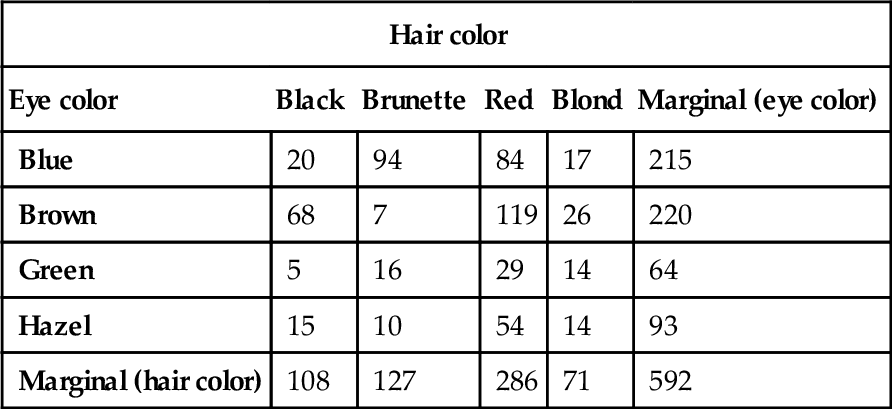
Data adapted from Snee (1974).
For data like these, we can ask a number of questions. We could wonder about one predictor at a time, and ask questions such as, “How much more frequent are brown-eyed people than hazel-eyed people?” or “How much more frequent are black-haired people than blond-haired people?” Those questions are analogous to main effects in ANOVA. But usually we display the joint counts specifically because we're interested in the relationship between the variables. We would like to know if the distribution of counts across one predictor is contingent upon the level of the other predictor. For example, does the distribution of hair colors depend on eye color, and, specifically, is the proportion of blond-haired people the same for brown-eyed people as for blue-eyed people? These questions are analogous to interaction contrasts in ANOVA.
24.1.2 Exponential link function
The model can be motivated two different ways. One way is simply to start with the two-way ANOVA model for combining nominal predictors, and find a way to map the predicted value to count data. The predicted μ from the ANOVA model (recall Equations 20.1 and 20.2, p. 584) could be any value from negative to positive infinity, but frequencies are non-negative. Therefore, we must transform the ANOVA predictions to non-negative values, while preserving order. The natural way to do this, mathematically, is with the exponential transformation. But this transformation only gets us to an underlying continuous predicted value, not to the probability of discrete counts. A natural candidate for the needed likelihood distribution is the Poisson (described later), which takes a non-negative value λ and gives a probability for each integer from zero to infinity. But this motivation may seem a bit arbitrary, even if there's nothing wrong with it in principle.
A different motivation starts by treating the cell counts as representative of underlying cell probabilities, and then asking whether the two nominal variables contribute independent influences to the cell probabilities. For example, in Table 24.1, there's a particular marginal probability that hair color is black, and a particular marginal probability that eye color is brown. If hair color and eye color are independent, then the joint probability of black hair and brown eyes is the product of the marginal probabilities. The attributes of hair color and eye color are independent if that relationship holds for every cell in the table. (![]() ecall the definition of independence in Section 4.4.2, p. 92.) Independence of hair color and eye color means that the proportion of black hair among brown-eyed people is the same as the proportion of black hair among blue-eyed people, and so on for all hair and eye colors.
ecall the definition of independence in Section 4.4.2, p. 92.) Independence of hair color and eye color means that the proportion of black hair among brown-eyed people is the same as the proportion of black hair among blue-eyed people, and so on for all hair and eye colors.
To check for independence of attributes, we need to estimate the marginal probabilities of the attributes. Denote the marginal (i.e., total) count of the rth row as yr, and denote the marginal count of the cth column as yc. Then the marginal proportions are yr/N and yc/N, where N is the total of the entire table. If the attributes are independent, then the predicted joint probability, ![]() , should equal the product of the marginal probabilities, which means
, should equal the product of the marginal probabilities, which means ![]() , hence
, hence ![]() . Because the models we've been dealing with involve additive combinations, not multiplicative combinations, we convert the multiplicative expression of independence into an additive expression by using the facts that log(a · b) = log(a) + log(b) and exp(log(x)) = x, as follows:
. Because the models we've been dealing with involve additive combinations, not multiplicative combinations, we convert the multiplicative expression of independence into an additive expression by using the facts that log(a · b) = log(a) + log(b) and exp(log(x)) = x, as follows:

If we abstract the form of Equation 24.1 away from the specific counts, we get the equation λr,c = exp + (β0 + βr + βc). The idea is that whatever are the values of the β's, the resulting λ's will obey multiplicative independence. An example is shown in Table 24.2. The choice of β's is shown in the margins of the table, and the resulting λ's are shown in the cells of the table. Notice that every row has the same relative probabilities, namely, 10, 100, and 1. In other words, the row and column attributes are independent.
Table 24.2
Example of exponentiated linear model with zero interaction
| β0 = 4.60517 | βc = 1 = 0 | βc = 2 = 2.30259 | βc = 3 = −2.30259 |
| βr = 1= 0 | 100 | 1000 | 10 |
| βr = 2= 2.30259 | 1000 | 10000 | 100 |
| βr = 3= −2.30259 | 10 | 100 | 1 |

Margins show the values of the β's, and cells show λr,c = exp (β0 + βr + βc) as in Equation 24.1. Notice that every row has the same relative probabilities, namely, 10, 100, 1. In other words, the row and column attributes are independent. Notice also that the row and column deflections sum to zero, as required by Equation 20.2 (p. 584).
We have dealt before with additive combinations of row and column influences, in the context of ANOVA. In ANOVA, β0 is a baseline representing the overall central tendency of the outcomes, and βr, is a deflection away from baseline due to being in the rth row, and βc is a deflection away from baseline due to being in the cth column. The deflections are constrained to sum to zero, as required by Equation 20.2 (p. 584), and the example in Table 24.2 respects this constraint.
In ANOVA, when the cell mean is not captured by an additive combination of row and column effects, we include interaction terms, denoted here as βr, c. The interaction terms are constrained so that every row and every column sums to zero: ![]() for all c and
for all c and ![]() for all r. The key idea is that the interaction terms in the model, which indicate violations of additivity in standard ANOVA, indicate violations of multiplicative independence in exponentiated ANOVA. To summarize, the model of the cell tendencies is Equation 24.1 extended with interaction terms:
for all r. The key idea is that the interaction terms in the model, which indicate violations of additivity in standard ANOVA, indicate violations of multiplicative independence in exponentiated ANOVA. To summarize, the model of the cell tendencies is Equation 24.1 extended with interaction terms:
with the constraints ![]() for all c, and
for all c, and ![]() for all rIf the researcher is interested in violations of independence, then the interest is on the magnitudes of the βr, c interaction terms, and specifically on meaningful interaction contrasts. The model is especially convenient for this purpose, because specific interaction contrasts can be investigated to determine in more detail where the nonindependence is arising.
for all rIf the researcher is interested in violations of independence, then the interest is on the magnitudes of the βr, c interaction terms, and specifically on meaningful interaction contrasts. The model is especially convenient for this purpose, because specific interaction contrasts can be investigated to determine in more detail where the nonindependence is arising.
24.1.3 Poisson noise distribution
The value of λr, c in Equation 24.2 is a cell tendency, not a predicted count per se. In particular, the value of λr, c can be any non-negative real value, but counts can only be integers. What we need is a likelihood function that maps the parameter value λr, c to the probabilities of possible counts. The Poisson distribution is a natural choice. The Poisson distribution is named after the French mathematician Simon-Denis Poisson (1781–1840) and is defined as
where y is a non-negative integer and λ is a non-negative real number. The mean of the Poisson distribution is λ. Importantly, the variance of the Poisson distribution is also λ (i.e., the standard deviation is ![]() ). Thus, in the Poisson distribution, the variance is completely yoked to the mean. Examples of the Poisson distribution are shown in Figure 24.1. Notice that the distribution is discrete, having masses only at non-negative integer values. Notice that the visual central tendency of the distribution does indeed correspond with λ. And notice that as λ increases, the width of the distribution also increases. The examples in Figure 24.1 use noninteger values of λ to emphasize that λ is not necessarily an integer, even though y is an integer.
). Thus, in the Poisson distribution, the variance is completely yoked to the mean. Examples of the Poisson distribution are shown in Figure 24.1. Notice that the distribution is discrete, having masses only at non-negative integer values. Notice that the visual central tendency of the distribution does indeed correspond with λ. And notice that as λ increases, the width of the distribution also increases. The examples in Figure 24.1 use noninteger values of λ to emphasize that λ is not necessarily an integer, even though y is an integer.

The Poisson distribution is often used to model discrete occurrences in time (or across space) when the probability of occurrence is the same at any moment in time (e.g., Sadiku & Tofighi, 1999). For example, suppose that customers arrive at a retail store at an average rate of 35 people per hour. Then the Poisson distribution, with λ = 35, is a model of the probability that any particular number of people will arrive in an hour. As another example, suppose that 11.2% of the students at the University of Delaware in the early 1970s had black hair and brown eyes, and suppose that an average of 600 students per term will fill out a survey. That means an average of 67.2 (= 11.2% · 600) students per term will indicate they have black hair and brown eyes. The Poisson distribution, p(y| λ = 67.2), gives the probability that any particular number of people will give that response in a term.
We will use the Poisson distribution as the likelihood function for modeling the probability of the observed count, yr,c, given the mean, λr,c, from Equation 24.2. The idea is that each particular r, c combination has an underlying average rate of occurrence, λr,c. We collect data for a certain period of time, during which we happen to observe particular frequencies, yr,c of each combination. From the observed frequencies, we infer the underlying average rates.
24.1.4 The complete model and implementation in JAGS
In summary, the preceding discussion says that the predicted tendency of the cell counts is given by Equation 24.2 (including the sum-to-zero constraints), and the probability of the observed cell count is given by the Poisson distribution in Equation 24.3. All we have yet to do is provide prior distributions for the parameters. Fortunately, we have already done this (at least structurally) for two-factor “ANOVA.” The resulting model is displayed in Figure 24.2. The top part shows the prior from two-factor “ANOVA,” reproduced from Figure 20.2 (p. 588). The mathematical expression in the middle of Figure 24.2 is the same as in Figure 20.2 except for the new exponential inverse-link function. The lower part of Figure 24.2 simply illustrates the Poisson noise distribution.

The model is implemented in JAGS as a variation on the model for two-factor “ANOVA.” As in that model, the sum-to-zero constraint is imposed by re-centering the deflection parameters that are found by MCMC without the constraint. The deflection parameters that are directly sampled by the MCMC process are denoted a1, a2, and a1a2, and the sum-to-zero versions are denoted b1, b2, and b1b2. To understand the following JAGS code, it is helpful to understand that the data file has one row per cell, such that the ith line of the data file contains the count y[i] from table row x1[i] and column x2[i]. The first part of the JAGS model specification directly implements the Poisson noise distribution and exponential inverse-link function:
The next part of the JAGS model specifies the prior distribution on the baseline and deflection parameters. The prior is supposed to be broad on the scale of the data, but we must be careful about what scale is being modeled by the baseline and deflections. The counts are being directly described by λ, but it is log(λ) being described by the baseline and deflections. Thus, the prior on the baseline and deflections should be broad on the scale of the logarithm of the data. To establish a generic baseline, consider that if the data points were distributed equally among the cells, the mean count would be the total count divided by the number of cells. The biggest possible standard deviation across cells would occur when all the counts were loaded into a single cell and all the other cells were zero. We take the logarithms of those values to define the following constants:
Those constants are used to set broad priors, as follows:
Near the end of the JAGS model specification, the baseline and deflections are recentered to respect the sum-to-zero constraints, exactly as was done for two-factor “ANOVA”:
Finally, a novel section of the model specification computes posterior predicted cell probabilities. Each cell mean (which was computed when re-centering for sum to zero) is exponentiated to compute the predicted count for each cell, and then the counts are normalized to compute the predicted proportion in each cell, denoted ppx1x2p. The predicted marginal proportions are also computed, as follows:
The model specification and other functions are defined in the file Jags-Ycount-Xnom2fac-MpoissonExp.R, and a high-level script that calls the functions is the file Jags-Ycount-Xnom2fac-MpoissonExp-Example.R.
24.2 Example: hair eye go again2
The analysis was run on the counts of eye and hair colors in Table 24.1. The posterior predicted cell proportions are shown in Figure 24.3. The top of Figure 24.3 is arrayed like the cells of Table 24.1, with the original counts in the titles of each panel. The data proportions (i.e., cell count divided by total count) are displayed as small triangles on the horizontal axis. In this case, the data proportions fall near the middles of the 95% HDIs in each cell. A nice feature of Bayesian analysis is the explicit posterior predictive uncertainty displayed in Figure 24.3.

Often we are interested in whether the attributes are independent, in the sense that the relative proportions of levels of one attribute do not depend on the level of the other attribute. As was explained earlier in the formal motivation of the model, lack of independence is captured by the model's interaction deflections. We consider any interaction contrasts that may be of interest. It is important to notice that independence refers to ratios of proportions, which corresponds to differences of underlying deflection parameters. In other words, it is not very meaningful to consider interaction contrasts of proportions; instead we consider interaction contrasts of deflection parameters. Suppose we are interested in the interaction contrast of blue eyes versus brown eyes for black hair versus blond hair. The lower panels of Figure 24.3 shows the corresponding differences of the underlying interaction deflection parameters. On the lower left is the difference of blue and brown eyes for black hair, which you can see has a negative value. This means that for black hair, the interaction deflection for brown eyes is larger than the interaction deflection for blue eyes, which makes intuitive sense insofar as we known brown eyes and black hair is a prominent combination. In the lower-middle panel of Figure 24.3 is the difference of blue and brown eyes for blond hair, which you can see has a positive value. Again this makes intuitive sense, as blue eyes and blond hair tend to go together. The lower-right panel shows the interaction contrast (i.e., the difference of differences), which is strongly nonzero. The nonzero interaction contrast means that the attributes are not independent.
The posterior distributions of differences in the lower row of Figure 24.3 are displayed with ![]() OPEs. When specifying a
OPEs. When specifying a ![]() OPE for the interaction deflection parameters, it is important to remember that the parameters are on the scale of the logarithm of the count. Thus, a difference of 0.1 corresponds to about a 10% change in the counts. In this case, the
OPE for the interaction deflection parameters, it is important to remember that the parameters are on the scale of the logarithm of the count. Thus, a difference of 0.1 corresponds to about a 10% change in the counts. In this case, the ![]() OPE was chosen arbitrarily merely for purposes of illustration.
OPE was chosen arbitrarily merely for purposes of illustration.
24.3 Example: interaction contrasts, shrinkage, and omnibus test
In this section, we consider some contrived data to illustrate aspects of interaction contrasts. Like the eye and hair data, the fictitious data have two attributes with four levels each. Figure 24.4 shows the cell labels and counts in the titles of the panels. The rows are the levels of attribute A (A1–A4) and the columns are the levels of attribute B (B1–B4). You can see that in the upper-left and lower-right quadrants, all the cells have counts of 22. In the upper-right and lower-left quadrants, all the cells have counts of11. This pattern of data suggests that there may be an interaction of the attributes, which is to say that the attributes are not independent.

When the JAGS program of the previous section is run on these data, it produces the posterior predictive distribution shown in Figure 24.4. You can see that cells with identical counts have nearly identical posterior predictive distributions, with variation between them caused only by randomness in the MCMC chain (a longer chain would yield less variation between cells with the same count). You can also see shrinkage in the predicted cell proportions: The modal predicted proportion for high-count cells is a little less than the data proportion, and the modal predicted proportion for the low-count cells is a little more than the data proportion. Exercise 24.2 has you examine shrinkage and its causes. In particular, you will find that if you change the structural assumptions about the prior, shrinkage is greatly reduced.
To assess the apparent lack of independence, we conduct interaction contrasts. One plausible interaction contrast involves the central four cells: ⟨A2, B2⟩, ⟨A2, B3⟩, ⟨A3, B2⟩, and ⟨A3, B3⟩. The interaction contrast asks whether the difference between A2 and A3 is the same at B2 as at B3. The result is in the bottom left of Figure 24.4, where it can be seen that the magnitude of the interaction contrast is non-zero but the 95% HDI nearly touches zero. Does this imply that there is not a sufficiently strong interaction and the attributes could be considered to be independent? No, because there are other interaction contrasts to consider. In particular, we can consider the interaction contrast that involves comparing the quadrants, averaging over the four cells in each quadrant. The result is in the bottom right of Figure 24.4, where it can be seen that the interaction contrast is clearly nonzero.
The model presented here has no way to conduct an “ominbus” test of interaction. However, like the ANOVA-style models presented in Chapters 19 and 20, it is easy to extend the model so it has an inclusion coefficient on the interaction deflections. The inclusion coefficient can have values of 0 or 1, and is given a Bernoulli prior. This extended model is fine in principle, but in practice the MCMC chain can be highly autocorrelated, and pseudo-priors may be helpful (as described in Section 10.3.2.1, p. 279). Also, the results must be carefully filtered so that steps in the chain when the inclusion coefficient is 1 are examined separately from steps in the chain when the inclusion coefficient is 0. Even when there is a high posterior probability that the inclusion coefficient is 1, we still must consider specific interaction contrasts to determine where the interaction “lives” in the data.
The traditional NHST omnibus test of independence for these type of data is the chi-square test, which I will not take the space here to explain. ![]() eaders who are already familiar with the chi-square test can compare its results to Bayesian interaction contrasts in Exercise 24.3.
eaders who are already familiar with the chi-square test can compare its results to Bayesian interaction contrasts in Exercise 24.3.
24.4 Log-linear models for contingency tables
This chapter only scratches the surface of methods for analyzing count data from nominal predictors. This type of data is often displayed as a table, and the counts in each cell are thought of as contingent upon the level of the nominal predictor. Therefore, the data are referred to as “contingency tables.” There can be more than two predictors, and models are generalized in the same way as ANOVA is generalized to more than two predictors. The formulation presented here has emphasized the inverse-link expressed as λ = exp(β0 + βr + βc + βr,c) in Equation 24.2, but this equation can also be written as log(λ) = β0 + βr + βc + βr,c. This latter form motivates the usual name for these models: log-linear models for contingency tables. This is the terminology to use when you want to explore these models more deeply. Agresti and Hitchcock (2005) provide a brief review of Bayesian log-linear models for contingency tables, but the method used in this chapter is not included, because the hierarchical ANOVA model was only popularized later (Gelman, 2005, 2006). For a description of Bayesian inference regarding contingency tables with a model like the one presented in this chapter but without the Gelman-style hierarchical prior, see Marin and Robert (2007, pp. 109–118) and Congdon (2005, p. 134 and p. 202).
24.5 Exercises
Look for more exercises at https://sites.google.com/site/doingbayesiandataanalysis/
Exercise 24.1
[Purpose: Trying the analysis on another data set.]
(A) A set of data from Snee (1974) reports counts of criminals on two attributes: the type of crime they committed and whether or not they regularly drink alcohol. Figure 24.5 shows the data in the titles of the panels. The data are in the file CrimeDrink.csv. ![]() un the analysis on the data using the script, Jags-Ycount-Xnom2fac-MpoissonExp-Example.R.
un the analysis on the data using the script, Jags-Ycount-Xnom2fac-MpoissonExp-Example.R.
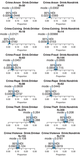
(B) What is the posterior estimate of the proportion of crimes that is committed by drinkers? Is the precision good enough to say that credibly more crimes are committed by drinkers than by nondrinkers? (This question is asking about a main-effect contrast.)
(C) What is the posterior estimate of the proportion of crimes that are fraud and the proportion that are violent (other than rape, which is a separate category in this data set)? Overall, is the precision good enough to say that those proportions are credibly different?
(D) Perform an interaction contrast of Fraud and Violence versus Drinker and Nondrink. What does this interaction contrast mean, in plain language?
Exercise 24.2
[Purpose: Exploring shrinkage of interaction contrasts.]
(A) Run the script Jags-Ycount-Xnom2fac-MpoissonExp-Example.R using the FourByFourCount.csv data with countMult=3. Figure 24.6 shows results, for your reference. Notice the shrinkage of cell-proportion estimates, and the funnel-shaped posteriors (like this: ![]() .) on interaction contrasts.
.) on interaction contrasts.

(B) Modify the model specification in Jags-Ycount-Xnom2fac-MpoissonExp.R as follows. Change
to
and run the analysis again. (Be sure to save the new version of Jags-Ycount-Xnom2fac-MpoissonExp.R so that the changes are sourced when you run the script.) Notice that the shrinkage disappears from the interaction contrast. Discuss why there is strong shrinkage of the interaction contrasts in the previous part but not in the version of this part.
(C) Continuing with the results of the previous part, notice that the modal cell proportions are smaller than the sample proportions. Despite the modes being less than the data proportions, verify that the posterior cell proportions really do sum to 1.0 on every step in the chain. Why are the modes of the marginals less than the sample proportions? (Hints: To extract the posterior cell proportions at every step, try something like the following.
Explain what that ![]() code does! The modes are less than the sample proportion because of marginalizing over the skew in the posterior.)
code does! The modes are less than the sample proportion because of marginalizing over the skew in the posterior.)
Exercise 24.3
[Purpose: Compare results of NHST chi-square test to results of Bayesian approach.] For this exercise, you must already be familiar with NHST chi-square tests. Also, you must have installed the reshape2 package, as described back in Section 3.6 (p. 56). Before doing the remainder of the exercise, load the reshape2 functions by typing the following at ![]() 's command line:
's command line:
(A) Let's do a traditional chi-square test of the hair-color eye-color data of Table 24.1. Type the following commands into ![]() :
:
Explain each line. What exactly do we conclude from this (omnibus) test? Do we know which subset of cells is responsible for the “significant” result? How might we find out? Does the omnibus test really tell us much?
(B) Let's do a traditional chi-square test of the data in Figures 24.4 and 24.6. Run the following lines three times, using countMult=11, countMult=7, and countMult=3.
Do the conclusions of the chi-square test match the conclusions of the Bayesian estimation? (You'll have to run the Bayesian estimation for countMult=7.) Can you compare an omnibus chi-square with the Bayesian interaction contrasts? Extra credit for overachievers: ![]() un the Bayesian estimations with a1a2SD set to a constant instead of estimated, as in Exercise 24.2.
un the Bayesian estimations with a1a2SD set to a constant instead of estimated, as in Exercise 24.2.