21.1.1 The model and implementation in JAGS

How can we describe the rise in the probability of 1's as height and weight increase in Figure 21.1? We will use a logistic function of a linear combination of the predictors. This type of model was introduced in Section 15.3.1.1 (p. 436), and in Figure 15.10 (p. 443). The idea is that a linear combination of metric predictors is mapped to a probability value via the logistic function, and the predicted 0's and 1's are Bernoulli distributed around the probability. Restated formally:

$\begin{array}{l}\mu =\text{logistic}\text{?}\left({\beta }_0+{\beta }_1{x}_1+{\beta }_2{x}_2\right)\\ y\sim \text{Bernoulli}\left(\mu \right)\end{array}$

where

$\text{logistic}\left(x\right)=\frac{1}{\left(1+\exp \left(-x\right)\right)}$

The intercept and slope parameters (i.e., β₀, β₁, and β₂) are given prior distributions in the usual ways, although the interpretation of logistic regression coefficients requires careful thought, as will be explained in Section 21.2.1.

A diagram of the model is presented in Figure 21.2. At the bottom of the diagram, each dichotomous y_i value comes from a Bernoulli distribution with a “bias” of μ_i. (Recall that I refer to the parameter in the Bernoulli distribution as the bias, regardless of its value. Thus, a coin with a bias value of 0.5 is fair.) The μ value is determined as the logistic function of the linear combination of predictors. Finally, the intercept and slope parameters are given conventional normal priors at the top of the diagram.

It can be useful to compare the diagram for multiple logistic regression (in Figure 21.2) with the diagram for robust multiple linear regression in Figure 18.4 (p. 515). The linear core of the model is the same in both diagrams. What differs across diagrams is the bottom of the diagram that describes y, because y is on different types of scales in the two models. In the present application (Figure 21.2), y is dichotomous and therefore is described as coming from a Bernoulli distribution. In the earlier application (Figure 18.4, p. 515), y was metric and therefore was described as coming from a t distribution (for robustness against outliers).

It is straight forward to compose JAGS (or Stan) code for the model in Figure 21.2. Before getting to the JAGS code itself, there are a couple more preliminary details to explain. First, as we did for linear regression, we will try to reduce autocorrelation in the MCMC chains by standardizing the data. This is done merely to improve the efficiency of the MCMC process, not out of logical necessity. The y values must be 0's and 1's and therefore are not standardized, but the predictor values are metric and are standardized. Recall from Equation 17.1 (p. 485) that we denote the standardized value of x as $z=\left(x-\overline{x}\right)/s_x$, where $\overline{x}$ is the mean of x and s_x is the standard deviation of x. And, recall from Equation 15.15 (p. 439) that the inverse logistic function is called the logit function. We standardize the data and let JAGS find credible parameter values, denoted ζ₀ and ζ_j, for the standardized data. We then transform the standardized parameter values to the original scale, as follows:

$\begin{array}{l}\text{logit}\left(\mu \right)={\zeta }_0+{\displaystyle \sum _j{\zeta }_j{z}_j}\\ \text{?}\text{?}\text{?}\text{?}\text{?}\text{?}\text{?}\text{?}\text{?}\text{?}\text{?}\text{?}\text{?}\text{?}\text{?}\text{?}\text{?}\text{?}\text{?}={\zeta }_0+{\displaystyle \sum _j{\zeta }_j\frac{x_j-{\overline{x}}_j}{s_{x_j}}}\\ \text{?}\text{?}\text{?}\text{?}\text{?}\text{?}\text{?}\text{?}\text{?}\text{?}\text{?}\text{?}\text{?}\text{?}\text{?}\text{?}\text{?}\text{?}=\underset{{\beta }_0}{\underbrace{{\zeta }_0-{\displaystyle \sum _j\frac{{\zeta }_j}{s_{x_j}}}{\overline{x}}_j}}+{\displaystyle \sum _j\underset{{\beta }_j}{\underbrace{\frac{{\zeta }_j}{s_{x_j}}}}{x}_j}\end{array}$

The transformation indicated by the underbraces in Equation 21.1 is applied at every step in the MCMC chain.

One more detail before getting to the JAGS code. In JAGS, the logistic function is called ilogit, for inverse logit. Recall from Section 15.3.1.1 (p. 436) that the inverse link function goes from the linear combination of predictors to the predicted tendency of the data, whereas the link function goes from the predicted tendency of the data to the linear combination of predictors. In this application, the link function is the logit. The inverse link function is, therefore, the inverse logit, abbreviated in JAGS as ilogit. The inverse link function is also, of course, the logistic. The ilogit notation helps distinguish the logistic function from the logistic distribution. We will not be using the logistic distribution, but just for your information, the logistic distribution is the probability density function which has a cumulative probability given by the logistic function. In other words, the logistic distribution is to the logistic function as the normal distribution is to the cumulative normal function in Figure 15.8 (p. 440). The logistic distribution is similar to the normal distribution but with heavier tails. Again, we will not be using the logistic distribution, and the point of this paragraph has been to explain JAGS' use of the term ilogit for the logistic function.

The JAGS code for the logistic regression model in Figure 21.2 is presented below. It begins with a data block that standardizes the data. Then the model block expresses the dependency arrows in Figure 21.2, and finally the parameters are transformed to the original scale using Equation 21.1:

# Standardize the data:
data {
 for ( j in 1:Nx ) {
 xm[j] <- mean(x[,j])
 xsd[j] <- sd(x[,j])
 for ( i in 1:Ntotal ) {
 zx[i,j] <- ( x[i,j] - xm[j] ) / xsd[j]
 }
 }
}
# Specify the model for standardized data:
model {
 for ( i in 1:Ntotal ) {
 # In JAGS, ilogit is logistic:
 y[i] ˜ dbern( ilogit( zbeta0 + sum( zbeta[1:Nx] * zx[i,1:Nx] ) ) )
 }
 # Priors vague on standardized scale:
 zbeta0 ˜ dnorm( 0 , 1/2ˆ2 )
 for ( j in 1:Nx ) {
 zbeta[j] ˜ dnorm( 0 , 1/2ˆ2 )
 }
 # Transform to original scale:
 beta[1:Nx] <- zbeta[1:Nx] / xsd[1:Nx]
 beta0 <- zbeta0 - sum( zbeta[1:Nx] * xm[1:Nx] / xsd[1:Nx] )
}

The line in the JAGS code that specified the Bernoulli distribution did not use a separate line for specifying μ_i because we did not want to record the μ_i values. If we wanted to, we would instead explicitly create μ_i as follows:

y[i] ˜ dbern( mu[i] )
mu[i] <- ilogit( zbeta0 + sum( zbeta[1:Nx] * zx[i,1:Nx] ) )

The complete program is in the file named Jags-Ydich-XmetMulti-Mlogistic.R, and the high-level script is the file named Jags-Ydich-XmetMulti-Mlogistic-Example.R.

21.1.2 Example: Height, weight, and gender

Consider again the data in Figure 21.4, which show the gender (male = 1, female = 0), height (in inches), and weight (in pounds) for 110 adults. We would like to predict gender from height and weight. We will first consider the results of using a single predictor, weight, and then consider the results of using both predictors.

Figure 21.3 shows the results of predicting gender from weight alone. The data are plotted as points that fall only at 0 or 1 on the y-axis. Superimposed on the data are logistic curves that have parameter values from various steps in the MCMC chain. The spread of the logistic curves indicates the uncertainty of the estimate; the steepness of the logistic curves indicates the magnitude of the regression coefficient. The 50% probability threshold is marked by arrows that drop down from the logistic curve to the x-axis, near a weight of approximately 160 pounds. The threshold is the x value at which μ = 0.5, which is x = −β₀/β₁. You can see that the logistic appears to have a clear positive (nonzero) rise as weight increases, suggesting that weight is indeed informative for predicting gender. But the rise is gentle, not steep: There is no sharp threshold weight below which most people are female and above which most people are male.

The lower panels of Figure 21.3 show the marginal posterior distribution on the parameters. In particular, the slope coefficient, β₁, has a mode larger than 0.03 and a 95% HDI that is well above zero (presumably by enough to exclude at least some non-zero ROPE). A later section will discuss how to interpret the numerical value of the regression coefficient.

Now we consider the results when using two predictors, namely both height and weight, as shown in Figure 21.4. The data are plotted as 1's and 0's with x₁ (weight) on the horizontal axis and x₂ (height) on the vertical axis. You can see from the scatter plot of points that weight and height are positively correlated. Superimposed on the data are credible level contours at which p(male) = 50%. Look back at Figure 21.1 (p. 623) for a picture of how a 50% level contour falls on a logistic surface. The 50% level contour is the set of x₁, x₂ values for which μ = 0.5, which is satisfied by x₂ = (–β₀/β₂) + (–β₁/β₂)x₁. On one side of the level contour there is less than 50% chance of being male, and on the other side of the level contour there is greater than 50% chance of being male, according to the model (not necessarily in reality). The spread of the credible level contours indicates the uncertainty in the parameter estimates. The perpendicular to the level contour indicates the direction in which probability changes the fastest. The angle of the level contours in Figure 21.4 suggests that the probability of being male increases rapidly as height goes up, but the probability of being male increases only a little as weight goes up. This interpretation is confirmed by the lower panels of Figure 21.4, which show the marginal posterior on the regression coefficients. In particular, the regression coefficient on weight has a modal value less than 0.02 and its 95% HDI essentially touches zero.

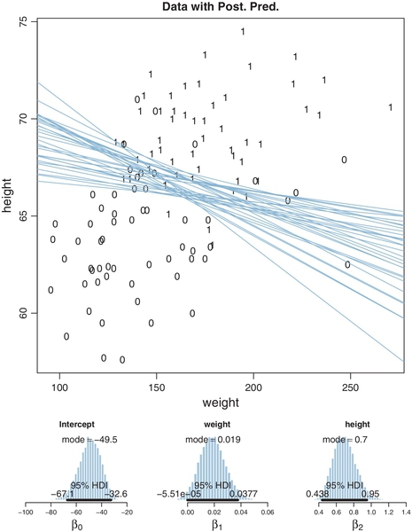
The regression coefficient on weight is smaller when height is included in the regression than when height is not included (compare Figure 21.4 with Figure 21.3). Why would this be? Perhaps you anticipated the answer: Because the predictors are correlated, and it's really height that's doing most of the predictive work in this case. When weight is the only predictor included, it has some predictive power because weight correlates with height, and height predicts gender. But when height is included as a second predictor, we find that the independent predictiveness of weight is relatively small. This issue of interpreting correlated predictors is the same here, in the context of logistic regression, as was discussed at length in Section 18.1.1 (p. 510) in the context of linear regression.

21.2.1 Log odds

When the logistic regression formula is written using the logit function, we have logit(μ) = β₀ + β₁x₁ + β₂x₂. The formula implies that whenever x₁ goes up by 1 unit (on the x₁ scale), then logit(μ) goes up by an amount β₁. And whenever x₂ goes up by 1 unit (on the x₂ scale), then logit(μ) goes up by an amount β₂. Thus, the regression coefficients are telling us about increases in logit(μ). To understand the regression coefficients, we need to understand logit(μ).

The logit function is the inverse of the logistic function. Formally, for 0 < μ < 1, logit(μ) = log (μ/(1 − μ)), where the logarithm is the natural logarithm, that is, the inverse of the exponential function. It's easy to verify through algebra that this expression for the logit really does make it the inverse of the logistic: If x = logit(μ) = log (μ/(1 − μ)), then μ = logistic(x) = 1/(1+exp(−x)) and vice versa. Now, in applications to logistic regression, μ is the probability that y = 1, and therefore we can write logit (μ) = logit (p(y = 1)) = log (p(y = 1)/ (1 − p(y = 1))) = log (p(y = 1)/p(y = 0)). The ratio, p(y = 1)/p(y = 0), is called the odds of outcome 1 to outcome 0, and therefore logit (μ) is the log odds of outcome 1 to outcome 0.

Combining the previous two paragraphs, we can say that the regression coefficients are telling us about increases in the log odds. Let's consider a numerical example. Rounding the modal values in Figure 21.4, suppose that β₀ = −50.0, β₁ = 0.02, and β₂ = 0.70.

• Consider a hypothetical person who weighs 160 pounds, that is, x₁ = 160. If that person were 63 inches tall, then the predicted probability of being male is logistic(β₀ + β₁x₁ + β₂x₂) = logistic(–50.0 + 0.02 · 160 + 0.70 · 63) = 0.063. That probability is a log odds of log(0.063/(1 − 0.063)) = −2.70. Notice the negative value of the log odds, which indicates the probability is less than 50%. If that person were 1 inch taller, at 64 inches, then the predicted probability of being male is 0.119, which has a log odds of −2.00. Thus, when x₂ was increased by 1 unit, the probability went up 0.056 (from 0.063 to 0.119), and the log odds increased 0.70 (from −2.70 to −2.00) which is exactly β₂.

• Again consider a hypothetical person who weighs 160 pounds, that is, x₁ = 160. Now consider an increase in height from 67 to 68 inches. If the person were 67 inches tall, then the predicted probability of being male is logistic(β₀ + β₁x₁ + β₂x₂) = logistic(–50.0 + 0.02 · 160 + 0.70 · 67) = 0.525. That probability is a log odds of log(0.525/(1 − 0.525)) = 0.10. Notice the positive value of the log odds, which indicates the probability is greater than 50%. If that person were 1 inch taller, at 68 inches, then the predicted probability of being male is 0.690, which has a log odds of 0.80. Thus, when x₂ was increased by 1 unit, the probability went up 0.165 (from 0.525 to 0.690), and the log odds increased 0.70 (from 0.10 to 0.80) which is exactly β₂.

The two numerical examples show that an increase of 1 unit of x_j increases the log odds by β_j. But a constant increase in log odds does not mean a constant increase in probability. In the first numerical example, the increase in probability was 0.056, but in the second numerical example, the increase in probability was 0.165.

Thus, a regression coefficient in logistic regression indicates how much a 1 unit change of the predictor increases the log odds of outcome 1. A regression coefficient of 0.5 corresponds to a rate of probability change of about 12.5 percentage points per x-unit at the threshold x value. A regression coefficient of 1.0 corresponds to a rate of probability change of about 24.4 percentage points per x-unit at the threshold x value. When x is much larger or smaller than the threshold x value, the rate of change in probability is smaller, even though the rate of change in log odds is constant.

21.2.2 When there are few 1's or 0's in the data

In logistic regression, you can think of the parameters as describing the boundary between the 0's and the 1's. If there are many 0's and 1's, then the estimate of the boundary parameters can be fairly accurate. But if there are few 0's or few 1's, the boundary can be difficult to identify very accurately, even if there are many data points overall.

In the data of Figure 21.1, involving gender (male, female) as a function of weight and height, there were approximately 50% 1's (males) and 50% 0's (females). Because there were lots of 0's and 1's, the boundary between them could be estimated relatively accurately. But many realistic data sets have only a small percentage of 0's or 1's. For example, suppose we are studying the incidence of heart attacks predicted by blood pressure. We measure the systolic blood pressure at the annual check-ups of a random sample of people, and then record whether or not they had a heart attack during the following year. We code not having a heart attack as 0 and having a heart attack as 1. Presumably the incidents of heart attack will be very few, and the data will have very few 1's. This dearth of 1's in the data will make it difficult to estimate the intercept and slope of the logistic function with much accuracy.

Figure 21.5 shows an example. For both panels, the x values of the data are identical, random values from a standardized normal distribution. For both panels, the y values were generated randomly from a Bernoulli distribution with bias given by a logistic function with the same slope, β₁ = 1. What differs between panels is where the threshold of the logistic falls relative to the mean of the x values. For the left panel, the threshold is at 3 (i.e., β₀ = −3), whereas for the right panel, the threshold is at 0. You can see that the data in the left panel have relatively few 1's (in fact, only about 7% 1's), whereas the data in the right panel have about 50% 1's. The right panel is analogous to the case of gender as a function of weight. The left panel is analogous to the case of heart attack as a function of blood pressure.

You can see in Figure 21.5 that the estimate of the slope (and of the intercept) is more certain in the right panel than in the left panel. The 95% HDI on the slope, β₁, is much wider in the left panel than in the right panel, and you can see that the logistic curves in the left panel have greater variation in steepness than the logistic curves in the right panel. The analogous statements hold true for the intercept parameter.

Thus, if you are doing an experimental study and you can manipulate the x values, you will want to select x values that yield about equal numbers of 0's and 1's for the y values overall. If you are doing an observational study, such that you cannot control any independent variables, then you should be aware that the parameter estimates may be surprisingly ambiguous if your data have only a small proportion of 0's or 1's. Conversely, when interpreting the parameter estimates, it helps to recognize when the threshold falls at the fringe of the data, which is one possible cause of relatively few 0's or 1's.

21.2.3 Correlated predictors

Another important cause of parameter uncertainty is correlated predictors. This issue was previously discussed at length, but the context of logistic regression provides novel illustration in terms of level contours.

Figure 21.6 shows a case of data with strongly correlated predictors. Both predictors have values randomly drawn from a standardized normal distribution. The y values are generated randomly from a Bernoulli distribution with bias given by slope parameters β₁ = 1 and β₂ = 1. The threshold falls in their midst, with β₀ = 0, so there are about half 0's and half 1's.

The posterior estimates of the parameter values are shown in Figure 21.6. In particular, notice that the 50% level contours (the threshold lines) are extremely ambiguous, with many different possible angles. The right panel shows strong anticorrelation of credible β₁ and β₂ values.

The same ambiguity can arise for correlations of multiple predictors, but higher-dimensional correlations are difficult to graph. As in the case of linear regression, it is important to consider the correlations of the predictors when interpreting the parameters of logistic regression. The high-level scripts display the predictor correlations on the $\mathrm{R}$ console.

21.2.4 Interaction of metric predictors

There may be applications in which it is meaningful to consider a multiplicative interaction of metric predictors. For example, in the case of predicting gender (male vs female) from weight and height, it could be that an additive combination of the predictors is not very accurate. For example, it might be that only the combination of tall and heavy is a good indicator of being male, while being tall but not heavy, or heavy but not tall, both indicate being female. This sort of conjunctive combination of predictors can be expressed by their multiplication (or other ways).

Figure 21.7 shows examples of logistic surfaces with multiplicative interaction of predictors. Within Figure 21.7, the title of each panel displays the formula being plotted. The left column of Figure 21.7 shows examples without interaction, for reference. The right column shows the same examples from the left column but with a multiplicative interaction included. In the top row, you can see that including the term +4x₁x₂ makes the logistic surface rise whenever x₁ and x₂ are both positive or both negative. In the bottom row, you can see that including a multiplicative interaction (with an adjustment of the intercept) produces the sort of conjunctive combination described in the previous paragraph. Thus, when either x₁ or x₂ is zero, the logistic surface is nearly zero, but when both predictors are positive, the logistic surface is high. Importantly, the 50% level contour is straight when there is no interaction, but is curved when there is interaction.

A key thing to remember when using an interaction term is that regression coefficients on individual predictors only indicate the slope when all the other predictors are set to zero. This issue was illustrated extensively in the context of linear regression in Section 18.2 (p. 525). Analogous points apply to logistic regression.

21.4.1 Single group

We start with the simplest, trivial case: A single group. In this case, we have several observed 0's and 1's, and our goal is to estimate the underlying probability of 1's. This is simply the case of estimating the underlying bias of a coin by observing several flips. The novelty here is that we treat it as a case of the generalized linear model, using a logistic function of a baseline.

Back in Chapter 6, we formalized this situation by denoting the bias of the coin as θ, and giving θ a beta prior. Thus, the model was y ∼ Bernoulli(θ) with θ ∼ dbeta(a, b). Now, the bias of the coin is denoted μ (instead of θ). The value of μ is given by a logistic function of a baseline, β₀. Thus, in the new model:

$y\sim \text{Bernoulli}\left(\mu \right)\text{?}\text{?}\text{?}\text{?}\text{?}\text{?}\text{with}\text{?}\text{?}\text{?}\text{?}\text{?}\mu \text{?}\text{=}\text{?}\text{logistic}\left({\beta }_0\right)$

The model expresses the bias in the coin in terms of β₀. When β₀ = 0, the coin is fair because μ = 0.5. When β₀ > 0, then μ > 0.5 and the coin is head biased. When β₀ < 0, then μ < 0.5 and the coin is tail biased. Notice that β₀ ranges from − ∞ to +∞, while μ ranges from 0 to 1. Therefore the prior on β₀ must also support −∞ to +∞. The conventional prior is a normal distribution:

${\beta }_0\sim \text{normal}\left(M_0,\text{?}{S}_0\right)$

When M₀ = 0, the prior distribution is centered at μ = 0.5. Figure 21.10 presents a diagram of the model, which should be compared with the beta prior in Figure 8.2 (p. 196).

Because μ is a logistic function of a normally distributed value β₀, it is not immediately obvious what the prior distribution of μ actually looks like. Figure 21.11 gives some examples. In each example, random values of β₀ were generated from its normal prior, and then those values of β₀ were converted to values of μ via the logistic function. The resulting values of μ were then plotted in a histogram. The histograms in Figure 21.11 are outlined by the exact mathematical form of the implied prior on μ, derived from the reparameterization formula explained in Section 25.3 (p. 729).²

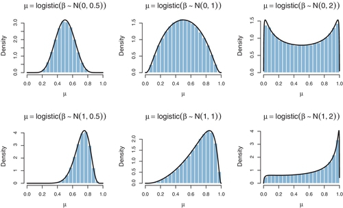
For some values of prior mean and standard deviation on β₀, the prior distribution of μ looks somewhat similar to a beta distribution. But there are many choices of prior mean and standard deviation that make the distribution of μ look nothing like a beta distribution. In particular, there is no choice of prior mean and standard deviation that give μ a uniform distribution. Also, while the beta-prior constants have a natural interpretation in terms of previously observed data (recall Section 6.2.1, p. 127), the normal-prior constants for the logistic mapping to μ are not as intuitive.

It is straight forward to convert the beta-prior program, Jags-Ydich-Xnom1subj-MbernBeta.R, to a version that uses the logistic of a baseline. (The new program could be called Jags-Ydich-Xnom1subj-Mlogistic.R.) The model specification from Jags-Ydich-Xnom1subj-MbernBeta.R is as follows:

model {
 for ( i in 1:Ntotal ) {
 y[i] ˜ dbern( theta )
 }
 theta ˜ dbeta(1,1)
}

The logistic version could instead use the following:

model {
 for ( i in 1:Ntotal ) {
 y[i] ˜ dbern( ilogit( b0 ) )
 }
 b0 ˜ dnorm( 0 , 1/2ˆ2)
}

The prior on β₀ was given a mean of M₀ = 0 and a standard deviation of S₀ = 2. Notice that the model specification, above, did not use a separate line to explicitly name μ. If you want to keep track of μ, you could do it after the fact by creating μ = logistic (β₀) at each step in the chain, or you could do it this way:

model {
 for ( i in 1:Ntotal ) {
 y[i] ˜ dbern( mu )
 }
 mu <- ilogit( b0 )
 b0 ˜ dnorm( 0 , 1/2ˆ2 )
}

Review Section 17.5.2 (p. 502) for tips about what other aspects of the program would need to be changed. For any given data set, the posterior distribution created by the logistic version of the program would not exactly match the posterior distribution created by the beta version of the program, because the prior distributions are not identical. You have the chance to try all this, hands on, in Exercise 21.2.

21.4.2 Multiple groups

The previous section discussed the trivial case of a single group, primarily for the purpose of introducing concepts. In the present section, we consider a more realistic case in which there are several groups. Moreover, instead of each “subject” within a group contributing a single dichotomous score, each subject contributes many dichotomous measures.

21.4.2.2 The model

The model we will use is diagrammed in Figure 21.12. The top part of the structure is based on the ANOVA-like model of Figure 19.2 (p. 558). It shows that the modal ability of position j, denoted ω_j, is a logistic function of a baseline ability β₀ plus a deflection for the position, β_[j]. The baseline and deflection parameters are given the usual priors for an ANOVA-style model.

The lower part of Figure 21.12 is based on the models of Figure 9.7 (p. 236) and Figure 9.13 (p. 252). The ability of position j, denoted ω_j, is the mode of a beta distribution that describes the spread of individual abilities within the position. The concentration of the beta distribution, denoted κ, is estimated and given a gamma prior. I've chosen to use a single concentration parameter to describe all groups simultaneously, by analogy to an assumption of homogeneity of variance in ANOVA. (Group-specific concentration parameters could be used, as shown in Figure 9.13, p. 252.) The ability of player i in position j is denoted μ_i|j. The number of hits by player i, out of N_i|j opportunities at bat, is denoted y_i|j, and is assumed to be a random draw from a binomial distribution with mean μ_i|j. We use the binomial distribution as a computational shortcut for multiple independent dichotomous events, not as a claim that the measuring event was conditional on fixed N, as was discussed is Section 9.4 (p. 249; see also Footnote 5, p. 249).

The model functions are in the file name Jags-Ybinom-Xnom1fac-Mlogistic.R, and the high-level script is the file named Jags-Ybinom-Xnom1fac-Mlogistic-Example.R. The JAGS model specification implements all the arrows in Figure 21.12. I hope that by this point in the book you can scan the JAGS model specification, below, and understand how each line of code corresponds with the arrows in Figure 21.12:

model {
 for ( i in 1:Ntotal ) {
 y[i] ˜ dbin( mu[i] , N[i] )
 mu[i] ˜ dbeta( omega[x[i]]*(kappa-2)+1, (1-omega[x[i]])*(kappa-2)+1 )
 }
 for ( j in 1:NxLvl ) {
 omega[j] <- ilogit( a0 + a[j] ) # In JAGS, ilogit is logistic
 a[j] ˜ dnorm( 0.0 , 1/aSigmaˆ2 )
 }
 a0 ˜ dnorm( 0.0 , 1/2ˆ2 )
 aSigma ˜ dgamma( 1.64 , 0.32 ) # mode=2, sd=4
 kappa <- kappaMinusTwo + 2
 kappaMinusTwo ˜ dgamma( 0.01 , 0.01 ) # mean=1 , sd=10 (generic vague)
 # Convert a0,a[] to sum-to-zero b0,b[] :
 for ( j in 1:NxLvl ) { m[j] <- a0 + a[j] } # cell means
 b0 <- mean( m[1:NxLvl] )
 for ( j in 1:NxLvl ) { b[j] <- m[j] - b0 }
}

The only novelty in the code, above, is the choice of constants in the prior for aSigma. Recall that aSigma represents σ_β in Figure 21.12, which is the standard deviation of the deflection parameters across groups. The gamma prior on aSigma was made broad on its scale. The reasonable values of σ_β are not very intuitive because they refer to standard deviations of deflections that are the inverse-logistic of probabilities. Consider two extreme probabilities near 0.001 and 0.999. The corresponding inverse-logistic values are about −6.9 and +6.9, which have a standard deviation of almost 10. This represents the high end of the prior distribution on σ_β, and more typical values will be around, say, 2. Therefore the gamma prior was given a mode of 2 and a standard deviation of 4. This is broad enough to have minimal influence on moderate amounts of data. You should change the prior constants if appropriate for your application.

21.4.2.3 Results

Each player's ratio of hits to at-bats is shown as a dot in Figure 21.13, with the dot size indicating the number of at-bats. Larger dots correspond to more data, and therefore should be more influential to the parameter estimation. The posterior predictive distribution is superimposed along the side of each group's data. The profiles are beta distributions from the model of Figure 21.12 with credible values of ω_j and κ. The beta distributions have their tails clipped so they span 95%. Each “moustache” is very thin, meaning that the estimate of the group modes is fairly certain. This high degree of certainty makes intuitive sense, because the data set is fairly large. The model assumed equal concentration in every group, which might be a poor description of the data. In particular, visual inspection of Figure 21.13 suggests that there might be greater variation within pitchers than within other positions.

Contrasts between positions are shown in the lower panels of Figure 21.13. The contrasts are shown for both the log odds deflection parameters (β_j or b) and the group modes (ω or omega). Compare the group-mode contrasts with the previously reported contrasts shown in Figure 9.14 (p. 256). They are very similar, despite the difference in model structure.

The present model focuses on descriptions at the group level, not at the individual-player level. Therefore the program does not have contrasts for individual players built in. But the JAGS model does record the individual-player estimates as mu[i], so contrasts of individual players can be conducted.

Which model is better, the ANOVA-style model of Figure 21.12 in this section, or the tower of beta distributions used in Figures 9.7 (p. 236) and 9.13 (p. 252)? The answer is: It depends. It depends on meaningfulness, descriptive adequacy, and generalizability. The tower of beta distributions might be more intuitively meaningful because the mode parameters of the beta distributions can be directly interpreted on the scale of the data, unlike the deflection parameters inside the logistic function. Descriptive adequacy for these data might demand that each group has its own concentration parameter, regardless of upper-level structure of the model. The ANOVA-style model may be more generalizable for applications that have multiple predictors, including covariates. Indeed, the top structure of Figure 21.12 can be changed to any combination of metric and nominal predictors that are of interest.