5.1 Bayes' rule

Thomas Bayes (1702-1761) was a mathematician and Presbyterian minister in England. His famous theorem was published posthumously in 1763, thanks to the extensive editorial efforts of his friend, Richard Price (Bayes & Price, 1763). The simple rule has vast ramifications for statistical inference, and therefore as long as his name is attached to the rule, we'll continue to see his name in textbooks.² But Bayes himself probably was not fully aware of these ramifications, and many historians argue that it is Bayes' successor, Pierre-Simon Laplace (1749-1827), whose name should really label this type of analysis, because it was Laplace who independently rediscovered and extensively developed the methods (e.g., Dale, 1999; McGrayne, 2011).

There is another branch of statistics, called frequentist, which does not use Bayes' rule for inference and decisions. Chapter 11 describes aspects of the frequentist approach and its perils. This approach is often identified with another towering figure from England who lived about 200 years later than Bayes, named Ronald Fisher (1890-1962). His name, or at least the first letter of his last name, is immortalized in one of the most common measures used in frequentist analysis, the F-ratio.³ It is curious and re-assuring that the overwhelmingly dominant Fisherian approach of the 20th century is giving way in the 21st century to a Bayesian approach that had its genesis in the 18th century (e.g., Lindley, 1975; McGrayne, 2011).⁴

5.1.2 Bayes' rule intuited from a two-way discrete table

Consider Table 5.1, which shows the joint probabilities of a row attribute and a column attribute, along with their marginal probabilities. In each cell, the joint probability p(r, c) is re-expressed by the equivalent form p(r | c) p(c) from the definition of conditional probability in Equation 5.3. The marginal probability p(r) is re-expressed by the equivalent form Σ_c*p(r | c*) p(c*), as was done in Equations 4.9 and 5.6. Notice that the numerator of Bayes' rule is the joint probability, p(r, c), and the denominator of Bayes' rule is the marginal probability, p(r). Looking at Table 5.1, you can see that Bayes' rule gets us from the lower marginal distribution, p(c), to the conditional distribution p(c | r) when focusing on row value r. In summary, the key idea is that conditionalizing on a known row value is like restricting attention to only the row for which that known value is true, and then normalizing the probabilities in that row by dividing by the row's total probability. This act of spatial attention, when expressed in algebra, yields Bayes' rule.

Table 5.1

A table for making Bayes’ rule not merely special but spatial

	Column
Row	…	c	…	Marginal
r	…	p(r, c) = p(r | c) p(c)	…	p(r) = Σc*p(r|c*)p(c*)
Marginal		p(c)

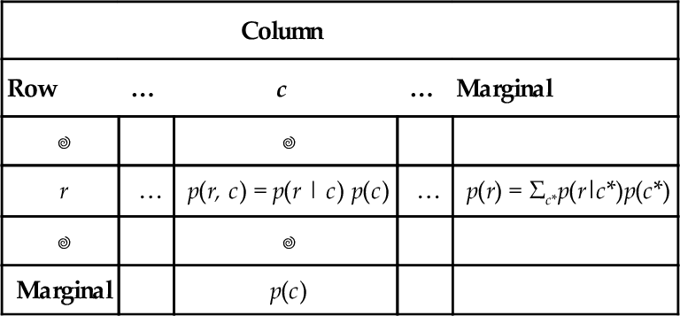
When conditionalizing on row value r, the conditional probability p(c | r) is simply the cell probability, p(r, c), divided by the marginal probability, p(r). When algebraically re-expressed as shown in the table, this is Bayes’ rule. Spatially, Bayes’ rule gets us from the lower marginal distribution, p(c), to the conditional distribution p(c | r) when focusing on row value r.

A concrete example of going from marginal to conditional probabilities was provided in the previous chapter, regarding eye color and hair color. Let's revisit it now. Table 5.2 shows the joint and marginal probabilities of various combinations of eye color and hair color. Without knowing anything about a person's eye color, all we believe about hair colors is expressed by the marginal probabilities of the hair colors, at the bottom of Table 5.2. However, if we are told that a randomly selected person's eyes are blue, then we know that this person comes from the “blue” row of the table, and we can focus our attention on that row. We compute the conditional probabilities of the hair colors, given the eye color, as shown in Table 5.3. Notice that we have gone from the “prior” (marginal) beliefs about hair color before knowing eye color, to the “posterior” (conditional) beliefs about hair color given the observed eye color. For example, without knowing the eye color, the probability of blond hair in this population is 0.21. But with knowing that the eyes are blue, the probability of blond hair is 0.45.

Table 5.2

Proportions of combinations of hair color and eye color

	Hair color
Eye color	Black	Brunette	Red	Blond	Marginal (Eye color)
Brown	0.11	0.20	0.04	0.01	0.37
Blue	0.03	0.14	0.03	0.16	0.36
Hazel	0.03	0.09	0.02	0.02	0.16
Green	0.01	0.05	0.02	0.03	0.11
Marginal (hair color)	0.18	0.48	0.12	0.21	1.0

Some rows or columns may not sum exactly to their displayed marginals because of rounding error from the original data. Data adapted from Snee (1974). This is a Table 4.1 duplicated here for convenience.

Table 5.3

Example of conditional probability

	Hair color
Eye color	Black	Brunette	Red	Blond	Marginal (Eye color)
Blue	0.03/0.36	0.14/0.36	0.03/0.36	0.16/0.36	0.36/0.36 = 1.0
	= 0.08	= 0.39	= 0.08	= 0.45

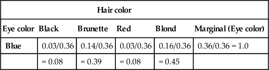
Of the blue-eyed people in Table 5.2, what proportion has hair color h? Each cell shows p(h|blue) = p(blue, h)/p(blue) rounded to two decimal points. This is a Table 4.2 duplicated here for convenience.

The example involving eye color and hair color illustrates conditional reallocation of credibility across column values (hair colors) when given information about a row value (eye color). But the example uses joint probabilities p(r, c) that are directly provided as numerical values, whereas Bayes' rule instead involves joint probabilities expressed as p(r|c) p(c), as shown in Equation 5.6 and Table 5.1. The next example provides a concrete situation in which it is natural to express joint probabilities as p(r|c) p(c).

Consider trying to diagnose a rare disease. Suppose that in the general population, the probability of having the disease is only one in a thousand. We denote the true presence or absence of the disease as the value of a parameter, θ, that can have the value θ = if disease is present in a person, or the value θ = if the disease is absent. The base rate of the disease is therefore denoted p(θ = ) = 0.001. This is our prior belief that a person selected at random has the disease.

Suppose that there is a test for the disease that has a 99% hit rate, which means that if a person has the disease, then the test result is positive 99% of the time. We denote a positive test result as T = +, and a negative test result as T =−. The observed test result is the datum that we will use to modify our belief about the value of the underlying disease parameter. The hit rate is expressed formally as p(T=+|θ = ) = 0.99. Suppose also that the test has a false alarm rate of 5%. This means that 5% of the time when the disease is absent, the test falsely indicates that the disease is present. We denote the false alarm rate as p(T=+|θ = ) = 0.05.

Suppose we sample a person at random from the population, administer the test, and it comes up positive. What is the posterior probability that the person has the disease? Mathematically expressed, we are asking, what is p(θ = | T=+)? Before determining the answer from Bayes' rule, generate an intuitive answer and see if your intuition matches the Bayesian answer. Most people have an intuition that the probability of having the disease is near the hit rate of the test (which in this case is 99%).

Table 5.4 shows how to conceptualize disease diagnosis as a case of Bayes' rule. The base rate of the disease is shown in the lower marginal of the table. Because the background probability of having the disease is p(θ = ) = 0.001, it is the case that the probability of not having the disease is the complement, p(θ = ) = 1-0.001 = 0.999. Without any information about test results, this lower marginal probability is our prior belief about a person having the disease.

Table 5.4

Joint and marginal probabilities of test results and disease states

For this example, the base rate of the disease is 0.001, as shown in the lower marginal. The test has a hit rate of 0.99 and a false alarm rate of 0.05, as shown in the row for T = +. For an actual test result, we restrict attention to the corresponding row of the table and compute the conditional probabilities of the disease states via Bayes’ rule.

Table 5.4 shows the joint probabilities of test results and disease states in terms of the hit rate, false alarm rate, and base rate. For example, the joint probability of the test being positive and the disease being present is shown in the upper-left cell as p(T = +,θ = ) = p(T = +|θ = ) p(θ = ) = 0.99 . 0.001. In other words, the joint probability of the test being positive and the disease being present is the hit rate of the test times the base rate of the disease. Thus, it is natural in this application to express the joint probabilities as p(row|column) p(column).

Suppose we select a person at random and administer the diagnostic test, and the test result is positive. To determine the probability of having the disease, we should restrict attention to the row marked T = + and compute the conditional probabilities of p(θ|T = +) via Bayes' rule. In particular, we find that

Yes, that's correct: Even with a positive test result for a test with a 99% hit rate, the posterior probability of having the disease is only 1.9%. This low probability is a consequence of the low-prior probability of the disease and the non-negligible false alarm rate of the test. A caveat regarding interpretation of the results: Remember that here we have assumed that the person was selected at random from the population, and there were no other symptoms that motivated getting the test. If there were other symptoms that indicated the disease, those data would also have to be taken into account.

To summarize the example of disease diagnosis: We started with the prior credibility of the two disease states (present or absent) as indicated by the lower marginal of Table 5.4. We used a diagnostic test that has a known hit rate and false alarm rate, which are the conditional probabilities of a positive test result for each disease state. When an observed test result occurred, we restricted attention to the corresponding row of Table 5.4 and computed the conditional probabilities of the disease states in that row via Bayes' rule. These conditional probabilities are the posterior probabilities of the disease states. The conditional probabilities are the re-allocated credibilities of the disease states, given the data.

5.2 Applied to parameters and data

The key application that makes Bayes' rule so useful is when the row variable represents data values and the column variable represents parameter values. A model of data specifies the probability of particular data values given the model's structure and parameter values. The model also indicates the probability of the various parameter values. In other words, a model specifies

$\begin{array}{l}\text{?}\text{?}p\left(\text{data values | parameters values}\right)\\ \text{along with the prior, }p\left(\text{parameters values}\right)\end{array}$

and we use Bayes' rule to convert that to what we really want to know, which is how strongly we should believe in the various parameter values, given the data:

$p\left(\text{parameters values | data values}\right)$

Comprehension can be aided by thinking about the application of Bayes' rule to data and parameters in terms of a two-way table, shown in Table 5.5. The columns of Table 5.5 correspond to specific values of the parameter, and the rows of Table 5.5 correspond to specific values of the data. Each cell of the table holds the joint probability of the specific combination of parameter value θ and data value D, denoted p(D,θ), and which we know can be algebraically re-expressed as p(D|θ) p(θ). The prior probability of the parameter values is the marginal distribution, p(θ), which appears in the lower margin of Table 5.5. Table 5.5 is merely Table 5.1 with its rows and columns renamed.

Table 5.5

Applying Bayes' Rule to data and parameters

	Model parameter
Data	…	θ value	…	Marginal
D value	…	p(D, θ) = p(D|θ) p(θ)	…	p(D) = Σθ*p(D|θ*) p(θ*)
Marginal	…	p(0)	…

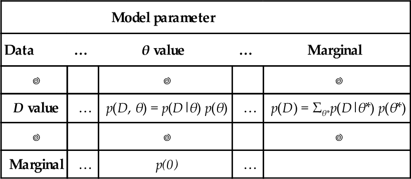
When conditionalizing on row value D, the conditional probability p(θ|D) is the cell probability p(D, θ) divided by the marginal probability p(D). When these probabilities are algebraically re-expressed as shown in the table, this is Bayes’ rule. This table is merely Table 5.1 with its rows and columns re-named.

When we observe a particular data value, D, we are restricting our attention to one specific row of Table 5.5, namely, the row corresponding to the observed value, D. The posterior distribution on θ is obtained by dividing the joint probabilities in that row by the row marginal, p(D). In other words, the posterior distribution on θ is obtained by conditionalizing on the row with the observed data value, and that operation is Bayes' rule.

It might help at this point to recapitulate the progression of ideas in the last few sections. In particular, Table 5.1 showed Bayes' rule in general form, using generic rows and columns. That table emphasized how the factors of Bayes' rule are positioned in a joint probability table, and how Bayes' rule amounts to moving attention from a margin of the table to a row of the table. Next, Table 5.4 showed a numerical example in which columns were underlying states of health (i.e., having or nor having a disease) and in which rows were observed data (i.e., testing positive or negative). That table emphasized a concrete case of the general form in Table 5.1. In disease diagnosis, we started with the marginal probabilities of the disease in Table 5.4, then re-allocated credibility across the disease states when the test result moved our attention to one row of the table. Finally, we re-expressed Table 5.1 as Table 5.5 by supposing that the rows are data values and the columns are parameter values. Bayes' rule is shifting attention from the prior, marginal distribution of the parameter values to the posterior, conditional distribution of parameter values in a specific datum's row. It is this form, in Table 5.5, that we will use throughout the remainder of the book. Additional examples will be presented very soon.

The factors of Bayes' rule have specific names that will be used regularly throughout the book, as indicated here:

$\begin{array}{lllll}\underset{\text{posterior}}{\underbrace{p\left(\theta |D\right)}}\hfill & =\hfill & \underset{\text{likelihood}}{\underbrace{p\left(\theta |D\right)}}\hfill & \underset{\text{prior}}{\underbrace{p\left(\theta \right)}}/\hfill & \underset{\text{evidence}}{\underbrace{p\left(D\right)}}\hfill \end{array}$

The denominator is

$p\left(D\right)\text{?}=\text{?}{\displaystyle \sum _{\theta *}p\left(D|{\theta }^{*}\right)p\left({\theta }^{*}\right)}$

where the superscript asterisk in θ* is merely a reminder that the denominator's θ* is distinct from the specific θ value in the numerator of Equation 5.7. The “prior,” p(θ), is the credibility of the θ values without the data D. The “posterior,” p(θ|D), is the credibility of θ values with the data D taken into account. The “likelihood” p(D|θ), is the probability that the data could be generated by the model with parameter value θ. The “evidence” for the model, p(D), is the overall probability of the data according to the model, determined by averaging across all possible parameter values weighted by the strength of belief in those parameter values.

The denominator of Bayes' rule, labeled in Equation 5.7 as the evidence for the model, is also called the marginal likelihood. The term “evidence” is intuitively suggestive and takes fewer syllables and characters than “marginal likelihood,” but the term “evidence” is also more ambiguous. The term “marginal likelihood” refers specifically to the operation of taking the average of the likelihood, p(D|θ), across all values of θ, weighted by the prior probability of θ. In this book, I will use the terms “evidence” and “marginal likelihood” interchangeably.

Up to this point, Bayes' rule has been presented only in the context of discrete-valued variables. It also applies to continuous variables, but probability masses become probability densities and sums become integrals. For continuous variables, the only change in Bayes' rule is that the marginal likelihood changes from the sum in Equation 5.8 to an integral:

$p\left(D\right)\text{?}=\text{?}{\displaystyle \int \text{d}{\theta }^{*}p\left(D|{\theta }^{*}\right)\text{?}p\left({\theta }^{*}\right)}$

where the superscript asterisk in θ* is merely a reminder that it is distinct from the specific θ value in Equation 5.7. This continuous-variable version of Bayes' rule is what we will deal with most often in real applications later in the book.⁵

5.3 Complete examples: Estimating bias in a coin

We will now consider an extensive set of examples that will build your understanding of how prior distributions and data interact to produce posterior distributions. These examples all involve estimating the underlying bias in a coin. Recall from Section 4.1.1 that we don't necessarily care about coins, per se, but coins represent things we do care about. When we observe the number of heads that result from flipping a coin, and we estimate its underlying probability of coming up heads, the exercise represents, for example, observing the number of correct responses on a multiple choice exam and estimating the underlying probability of being correct, or observing the number of headaches cured by a drug and estimating the underlying probability of curing.

A note about terminology: When I refer to the “bias” in a coin, I will sometimes be referring to its underlying probability of coming up heads. Thus, when a coin is fair, it has a “bias” of 0.50. Other times, I might use the term “bias” in its colloquial sense of a departure from fairness, as in “head biased” or “tail biased.” Although I will try to be clear about which meaning is intended, there will be times that you will have to rely on context to determine whether “bias” means the probability of heads or departure from fairness. I hope the ambiguity does not bias you against me.

Recall from Section 2.3 (p. 25) that the first step in Bayesian data analysis is identifying the type of data being described. In this case, the data consist of heads and tails. We will denote the outcome of a flip as y. When the outcome is heads, we say y = 1, and when the outcome is tails, we say y = 0. Although we are denoting the outcome with numerical values for mathematical convenience later, it should be remembered that heads and tails are merely categorical, with no metric attributes. In particular, heads is not greater than tails, nor are heads and tails separated by a distance of 1 unit, nor is heads something while tails is nothing. The values of 1 and 0 are used merely as labels with useful algebraic properties in subsequent formulas.

The next step in Bayesian data analysis is creating a descriptive model with meaningful parameters. We denote the underlying probability of coming up heads as p(y = 1). We want to describe that underlying probability with some meaningfully parameterized model. We will use a particularly simple model and directly describe the underlying probability of heads as the value of the parameter θ (Greek letter theta). This idea can be written formally as p(y = 1 |θ) = θ, which could be said aloud this way: “The probability that the outcome is heads, given a value of parameter θ is the value of θ.” Notice that this definition requires that the value of θ is between 0 and 1. A nice quality of this model is that θ is intuitively meaningful: its value is directly interpretable as the probability that the coin comes up heads.⁶

For our formal model, we need a mathematical expression of the likelihood function in Bayes' rule (Equation 5.7). We already have an expression for the probability of heads, namely p(y = 1|θ) = θ, but what about the probability of tails? A moment's thought suggests that the probability of tails is simply the complement of the probability of heads, because heads and tails are the only possible outcomes. Therefore, p (y = 0 | θ) = 1−θ. We can combine the equations for the probabilities of heads and tails into a single expression:

$p\left(y|\theta \right)={\theta }^y{\left(1-\theta \right)}^{\left(1-y\right)}$

Notice that when y = 1, Equation 5.10 reduces to p(y = 1|θ) = θ, and when y = 0, Equation 5.10 reduces to p(y = 0|θ) = 1 − θ. The probability distribution expressed by Equation 5.10 is called the Bernoulli distribution, named after the mathematician Jacob Bernoulli (1655-1705).⁷

As an aside, from Equation 5.10 we can also figure out the formula for the likelihood of a whole set of outcomes from multiple flips. Denote the outcome of the ith flip as y_iand denote the set of outcomes as {y_i}. We assume that the outcomes are independent of each other, which means that the probability of the set of outcomes is the multiplicative product of the probabilities of the individual outcomes. Therefore, we derive the following formula for the probability of the set of outcomes:

$\begin{array}{cccc}p\left(\left\{y_i\right\}|\theta \right)& =& {\displaystyle \prod _{i}p\left(y_i|\theta \right)}\hfill & \hfill \text{by assumption of independence}\\ & =& {\displaystyle \prod _i{\theta }^{yi}{\left(1-\theta \right)}^{\left(1-y_i\right)}}\hfill & \hfill \text{from Equation }5.10\\ & =& \theta {\displaystyle {\sum }_i{y}_i\left(1-\theta \right){\displaystyle {\sum }_i\left(1-y_i\right)}}\hfill & \hfill \text{by algebra}\\ & =& {\theta }^{\#\text{heads}}{\left(1-\theta \right)}^{\#\text{tails}}\hfill & \end{array}$

The final line of Equation 5.11 is a consequence of the fact that y_i is 1 for heads and y_i is 0 for tails; hence, Σ_iy_i = #heads and Σ_i1–y_i = #tails. Later, we will also refer to #heads as z, the number of flips as N, and hence the #tails as N − z. Equation 5.11 will be useful later for numerical computations of Bayes' rule.

Now that we have defined the likelihood function in Equation 5.10, the next step (recall Section 2.3, p. 25) is establishing a prior distribution over the parameter values. At this point, we are merely building intuitions about Bayes' rule, and therefore, we will use an unrealistic but illustrative prior distribution. For this purpose, we suppose that there are only a few discrete values of the parameter θ that we will entertain, namely θ = 0.0, θ = 0.1, θ = 0.2, θ = 0.3, and so forth up to θ = 1.0. You can think of this as meaning that there is a factory that manufactures coins, and the factory generates coins of only those 11 types: Some coins have θ = 0.0, some coins have θ = 0.1, some coins have θ = 0.2, and so forth. The prior distribution indicates what we believe about the factory's production of those types. Suppose we believe that the factory tends to produce fair coins, with θ near 0.5, and we assign lower prior credibility to biases far above or below θ = 0.5. One exact expression of this prior distribution is shown in the top panel of Figure 5.1. That panel shows a bar plotted at each candidate value of θ, with the height of the bar indicating the prior probability, p(θ). You can see that the heights have a triangular shape, with the peak of the triangle at θ = 0.5, and the heights decreasing toward either extreme, such that p(θ =0) = 0 and p(θ =1) = 0. Notice that this graph is just like the Sherlock Holmes examples in Figure 2.1 (p. 17), the exoneration example in Figure 2.2 (p. 18), and especially the normal-means example in Figure 2.3 (p. 21), where we considered a discrete set of candidate possibilities.

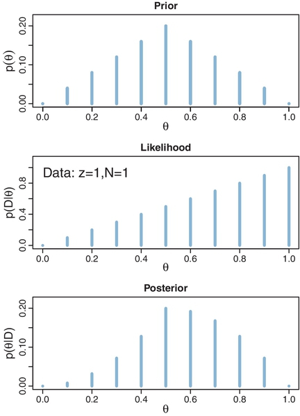
The next steps of Bayesian data analysis (recall Section 2.3, p. 25) are collecting the data and applying Bayes' rule to re-allocate credibility across the possible parameter values. Suppose that we flip the coin once and observe heads. In this case, the data D consist of a single head in a single flip, which we annotate as y = 1 or, equivalently, z = 1 with N = 1. From the formula for the likelihood function in Equation 5.10, we see that for these data the likelihood function becomes p(D|θ) = θ. The values of this likelihood function are plotted at the candidate values of θ in the middle panel of Figure 5.1. For example, the bar at θ = 0.2 has height p(D|θ) = 0.2, and the bar at θ = 0.9 has height p(D|θ) = 0.9.

The posterior distribution is shown in the lower panel of Figure 5.1. At each candidate value of θ the posterior probability is computed from Bayes' rule (Equation 5.7) as the likelihood at θ times the prior at θ divided by p(D). For example, consider θ = 0.2, scanning vertically across panels. In the lower panel at θ = 0.2, the posterior probability is the likelihood from the middle panel at θ = 0.2 times the prior in the upper panel at θ = 0.2, divided by the sum, p(D) = Σ_θ*p(D | θ*) p(θ*). This relationship is true at all values of θ.

Notice that the overall contour of the posterior distribution is different from the prior distribution. Because the data showed a head, the credibility of higher θ values has increased. For example, in the prior distribution, p(θ = 0.4) equals p(θ = 0.6), but in the posterior distribution, p(θ = 0.4|D) is less than p(θ = 0.6|D). Nevertheless, the prior distribution has a notable residual effect on the posterior distribution because it involves only a single flip of the coin. In particular, despite the data showing 100% heads (in a sample consisting of a single flip), the posterior probability of large θ values such as 0.9 is low. This illustrates a general phenomenon in Bayesian inference: The posterior is a compromise between the prior distribution and the likelihood function. Sometimes this is loosely stated as a compromise between the prior and the data. The compromise favors the prior to the extent that the prior distribution is sharply peaked and the data are few. The compromise favors the likelihood function (i.e., the data) to the extent that the prior distribution is flat and the data are many. Additional examples of this compromise are explained next.

5.3.1 Influence of sample size on the posterior

Suppose we fill in the candidate values of θ with 1,001 options, from 0.000, 0.001, 0.002, up to 1.000. Figure 5.1 would then be filled in with a dense forest of vertical bars, side by side with no visible space between them. But Bayes' rule applies the same as before, despite there being 1,001 candidate values of θ instead of only 11. Figure 5.2 shows two cases in which we start with the triangular prior used previously, but now filled in with 1,001 candidate values for θ. In the left side of Figure 5.2, the data consist of 25% heads for a small sample of N = 4 flips. In the right side of Figure 5.2, the data again consist of 25% heads, but for a larger sample of N = 40 flips. Notice that the likelihood functions in both cases have their modal (i.e., maximal) value at θ = 0.25. This is because the probability of 25% heads is maximized in the likelihood function (Equation 5.11) when θ = 0.25. Now inspect the posterior distributions at the bottom of Figure 5.2. For the small sample size, on the left, the mode (peak) of the posterior distribution is at θ = 0.40, which is closer to the mode of the prior distribution (at 0.5) than the mode of the likelihood function. For the larger sample size, on the right, the mode of the posterior distribution is at θ = 0.268, which is close to the mode of the likelihood function. In both cases, the mode of the posterior distribution is between the mode of the prior distribution and the mode of the likelihood function, but the posterior mode is closer to the likelihood mode for larger sample sizes.

Notice also in Figure 5.2 that the width of the posterior highest density intervals (HDI) is smaller for the larger sample size. Even though both samples of data showed 25% heads, the larger sample implied a smaller range of credible underlying biases in the coin. In general, the more data we have, the more precise is the estimate of the parameter(s) in the model. Larger sample sizes yield greater precision or certainty of estimation.

5.3.2 Influence of the prior on the posterior

In Figure 5.3, the left side is the same small sample as the left side of Figure 5.2, but the prior in Figure 5.3 is flatter. Notice that the posterior distribution in Figure 5.3 is very close to the likelihood function, despite the small sample size, because the prior is so flat. In general, whenever the prior distribution is relatively broad compared with the likelihood function, the prior has fairly little influence on the posterior. In most of the applications in this book, we will be using broad, relatively flat priors.

The right side of Figure 5.3 is the same larger sample as the right side of Figure 5.2, but the prior in Figure 5.3 is sharper. In this case, despite the fact that the sample has a larger size of N = 40, the prior is so sharp that the posterior distribution is noticeably influenced by the prior. In real applications, this is a reasonable and intuitive inference, because in real applications a sharp prior has been informed by genuine prior knowledge that we would be reluctant to move away from without a lot of contrary data.

In other words, Bayesian inference is intuitively rational: With a strongly informed prior that uses a lot of previous data to put high credibility over a narrow range of parameter values, it takes a lot of novel contrary data to budge beliefs away from the prior. But with a weakly informed prior that spreads credibility over a wide range of parameter values, it takes relatively little data to shift the peak of the posterior distribution toward the data (although the posterior will be relatively wide and uncertain).

These examples have used arbitrary prior distributions to illustrate the mechanics of Bayesian inference. In real research, the prior distributions are either chosen to be broad and noncommittal on the scale of the data or specifically informed by publicly agreed prior research. As was the case with disease diagnosis in Table 5.4 (p. 104), it can be advantageous and rational to start with an informed prior, and it can be a serious blunder not to use strong prior information when it is available. Prior beliefs should influence rational inference from data, because the role of new data is to modify our beliefs from whatever they were without the new data. Prior beliefs are not capricious and idiosyncratic and covert, but instead are based on publicly agreed facts or theories. Prior beliefs used in data analysis must be admissible by a skeptical scientific audience. When scientists disagree about prior beliefs, the analysis can be conducted with multiple priors, to assess the robustness of the posterior against changes in the prior. Or, the multiple priors can be mixed together into a joint prior, with the posterior thereby incorporating the uncertainty in the prior. In summary, for most applications, specification of the prior turns out to be technically unproblematic, although it is conceptually very important to understand the consequences of one's assumptions about the prior.

5.4 Why bayesian inference can be difficult

Determining the posterior distribution directly from Bayes' rule involves computing the evidence (a.k.a. marginal likelihood) in Equations 5.8 and 5.9. In the usual case of continuous parameters, the integral in Equation 5.9 can be impossible to solve analytically. Historically, the difficulty of the integration was addressed by restricting models to relatively simple likelihood functions with corresponding formulas for prior distributions, called conjugate priors, that “played nice” with the likelihood function to produce a tractable integral. A couple cases of this conjugate-prior approach will be illustrated later in the book, but this book will instead emphasize the flexibility of modern computer methods. When the conjugate-prior approach does not work, an alternative is to approximate the actual functions with other functions that are easier to work with, and then show that the approximation is reasonably good under typical conditions. This approach goes by the name “variational approximation.” This book does not provide any examples of variational approximation, but see Grimmer (2011) for an overview and pointers to additional sources.

Instead of analytical mathematical approaches, another class of methods involves numerical approximation of the integral. When the parameter space is small, one numerical approximation method is to cover the space with a comb or grid of points and compute the integral by exhaustively summing across that grid. This was the approach we used in Figures 5.2 and 5.3, where the domain of the parameter θ was represented by a fine comb of values, and the integral across the continuous parameter θ was approximated by a sum over the many discrete representative values. This method will not work for models with many parameters, however. In many realistic models, there are dozens or even hundreds of parameters. The space of possibilities is the joint parameter space involving all combinations of parameter values. If we represent each parameter with a comb of, say, 1,000 values, then for P parameters there are 1,000^P combinations of parameter values. When P is even moderately large, there are far too many combinations for even a modern computer to handle.

Another kind of approximation involves randomly sampling a large number of representative combinations of parameter values from the posterior distribution. In recent decades, many such algorithms have been developed, generally referred to as Markov chain Monte Carlo (MCMC) methods. What makes these methods so useful is that they can generate representative parameter-value combinations from the posterior distribution of complex models without computing the integral in Bayes' rule. It is the development of these MCMC methods that has allowed Bayesian statistical methods to gain practical use. This book focuses on MCMC methods for realistic data analysis.

5.5 Appendix: R code for figures 5.1, 5.2, etc.

Figures 5.1, 5.2, etc., were created with the program BernGrid.R, which is in the program files for this book. The file name refers to the facts that the program estimates the bias in a coin using the Bernoulli likelihood function and a grid approximation for the continuous parameter. The program BernGrid.R defines a function named BernGrid. Function definitions and their use were explained in Section 3.7.3 (p. 64). The BernGrid function requires three user-specified arguments and has several other arguments with function-supplied default values. The three user-specified arguments are the grid of values for the parameter, Theta, the prior probability masses at each of those values, pTheta, and the data values, Data, which consists of a vector of 0's and 1's. Before calling the BernGrid function, its definition must be read into $\text{R}$ using the source command. The program also uses utility functions defined in DBDA2E-utilities.R.Here is an example of how to use BernGrid, assuming that $\text{R}$'s working directory contains the relevant programs:

source("DBDA2E-utilities.R") # Load definitions of graphics functions etc.
source("BernGrid.R")  # Load the definition of the BernGrid function
Theta = seq(0, 1, length=1001)  # Specify fine comb for Theta.
pTheta = pmin(Theta, 1-Theta)  # Triangular shape for pTheta.
pTheta = pTheta/sum(pTheta)  # Make pTheta sum to 1.0
Data = c(rep(0,3),rep(1,1))  # Same as c(0,0,0,1). 25% heads with N=4.
openGraph(width=5,height=7) # Open a graphics window.
posterior = BernGrid(Theta, pTheta, Data, plotType="Bars",
 showCentTend="Mode", showHDI=TRUE, showpD=FALSE)
saveGraph(file="BernGridExample",type="jpg")

The first two lines above use the source function to read in $\text{R}$ commands from files. The source function was explained in Section 3.7.2. The next line uses the seq command to create a fine comb of θ values spanning the range from 0 to 1. The seq function was explained in Section 3.4.1.3.

The next line uses the pmin command to establish a triangular-shaped prior on the Theta vector. The pmin function has not been used previously in this book. To learn what it does, you could type ?pmin at the $\text{R}$ command line. There you will find that pmin determines the component-wise minimum values of vectors, instead of the single minimum of all components together. For example, pmin(c(0,.25,.5,.75, 1), c(1,.75,.5,.25, 0)) yields c(0,.25,.5,.25,0). Notice how the values in the result go up then down, to form a triangular trend. This is how the triangular trend on pTheta is created.

The next line uses the sum command. It takes a vector argument and computes the sum of its components. The next line uses the rep function, which was explained in Section 3.4.1.4, to create a vector of zeros and ones that represent the data.

The BernGrid function is called in the penultimate line. Its first three arguments are the previously defined vectors, Theta, pTheta, and Data. The next arguments are optional. The plotType argument can be "Bars" (the default) or "Points". Try running it both ways to see the effect of this argument. The showCentTend argument specifies which measure of central tendency is shown and can be "Mode" or "Mean" or "None" (the default). The showHDI argument can be TRUE or FALSE (the default). The mass of the HDI is specified by the argument HDImass, which has a default value of 0.95. You will notice that for sparse grids on θ, it is usually impossible to span grid values that exactly achieve the desired HDI, and therefore, the bars that minimally exceed the HDI mass are displayed. The showpD argument specifies whether or not to display the value of the evidence from Equation 5.8. We will have no use for this value until we get into the topic of model comparison, in Section 10.1.

The previous paragraphs explained how to use the BernGrid function. If you want to know its internal mechanics, then you can open the function definition, BernGrid.R, in $\text{R}$Studio's editing window. You will discover that the vast majority of the program is devoted to producing the graphics at the end, and the next largest part is devoted to checking the user-supplied arguments for consistency at the beginning. The Bayesian part of the program consists of only a few lines:

# Create summary values of Data
z = sum(Data) # number of 1's in Data
N = length(Data)
# Compute the Bernoulli likelihood at each value of Theta:
pDataGivenTheta = Thetaˆz * (1-Theta)ˆ(N-z)
# Compute the evidence and the posterior via Bayes' rule:
pData = sum(pDataGivenTheta * pTheta)
pThetaGivenData = pDataGivenTheta * pTheta / pData

The Bernoulli likelihood function in the $\text{R}$ code is in the form of Equation 5.11. Notice that Bayes' rule appears written in the $\text{R}$ code very much like Equations 5.7 and 5.8.

5.6 Exercises

Look for more exercises at https://sites.google.com/site/doingbayesiandataanalysis/