7.2.1 A politician stumbles upon the Metropolis algorithm

Suppose an elected politician lives on a long chain of islands. He is constantly traveling from island to island, wanting to stay in the public eye. At the end of a grueling day of photo opportunities and fundraising,² he has to decide whether to (i) stay on the current island, (ii) move to the adjacent island to the west, or (iii) move to the adjacent island to the east. His goal is to visit all the islands proportionally to their relative population, so that he spends the most time on the most populated islands, and proportionally less time on the less populated islands. Unfortunately, he holds his office despite having no idea what the total population of the island chain is, and he doesn't even know exactly how many islands there are! His entourage of advisers is capable of some minimal information gathering abilities, however. When they are not busy fundraising, they can ask the mayor of the island they are on how many people are on the island. And, when the politician proposes to visit an adjacent island, they can ask the mayor of that adjacent island how many people are on that island.

The politician has a simple heuristic for deciding whether to travel to the proposed island: First, he flips a (fair) coin to decide whether to propose the adjacent island to the east or the adjacent island to the west. If the proposed island has a larger population than the current island, then he definitely goes to the proposed island. On the other hand, if the proposed island has a smaller population than the current island, then he goes to the proposed island only probabilistically, to the extent that the proposed island has a population as big as the current island. If the population of the proposed island is only half as big as the current island, the probability of going there is only 50%.

In more detail, denote the population of the proposed island as P_proposed, and the population of the current island as P_current. Then he moves to the less populated island with probability p_move=P_proposed/P_current. The politician does this by spinning a fair spinner marked on its circumference with uniform values from zero to one. If the pointed-to value is between zero and p_move, then he moves.

What's amazing about this heuristic is that it works: In the long run, the probability that the politician is on any one of the islands exactly matches the relative population of the island!

7.2.2 A random walk

Let's consider the island hopping heuristic in a bit more detail. Suppose that there are seven islands in the chain, with relative populations as shown in the bottom panel of Figure 7.2. The islands are indexed by the value θ, whereby the leftmost, western island is θ = 1 and the rightmost, eastern island is θ = 7. The relative populations of the islands increase linearly such that P(θ) = θ. Notice that uppercase P() refers to the relative population of the island, not its absolute population and not its probability mass. To complete your mental picture, you can imagine islands to the left of 1 and to the right of 7 that have populations of zero. The politician can propose to jump to those islands, but the proposal will always be rejected because the population is zero.

The middle panel of Figure 7.2 shows one possible trajectory taken by the politician. Each day corresponds to one-time increment, indicated on the vertical axis. The plot of the trajectory shows that on the first day (t = 1), the politician happens to start on the middle island in the chain, hence θ_current=4. To decide where to go on the second day, he flips a coin to propose moving either one position left or one position right. In this case, the coin proposed moving right, hence θ_proposed = 5. Because the relative population at the proposed position is greater than the relative population at the current position (i.e., P(5) > P(4)), the proposed move is accepted. The trajectory shows this move, because when t = 2, then θ = 5.

Consider the next day, when t = 2 and θ = 5. The coin flip proposes moving to the left. The probability of accepting this proposal is p_move = P (θ_proposed)/P (θ_current) = 4/5 = 0.80. The politician then spins a fair spinner that has a circumference marked from 0 to 1, which happens to come up with a value greater than 0.80. Therefore, the politician rejects the proposed move and stays at the current island. Hence the trajectory shows that θ is still 5 when t = 3. The middle panel of Figure 7.2 shows the trajectory for the first 500 steps in this random walk across the islands. The scale of the time step is plotted logarithmically so you can see the details of the early steps but also see the trend of the later steps. There are many thousands of steps in the simulation.

The upper panel of Figure 7.2 shows a histogram of the frequencies with which each position is visited during this junket. Notice that the sampled relative frequencies closely mimic the actual relative populations in the bottom panel! In fact, a sequence generated this way will converge, as the sequence gets longer, to an arbitrarily close approximation of the actual relative probabilities.

7.2.3 General properties of a random walk

The trajectory shown in Figure 7.2 is just one possible sequence of positions when the movement heuristic is applied. At each time step, the direction of the proposed move is random, and if the relative probability of the proposed position is less than that of the current position, then acceptance of the proposed move is also random. Because of the randomness, if the process were started over again, then the specific trajectory would almost certainly be different. $R$egardless of the specific trajectory, in the long run the relative frequency of visits mimics the target distribution.

Figure 7.3 shows the probability of being in each position as a function of time. At time t = 1, the politician starts at θ = 4. This starting position is indicated in the upper-left panel of Figure 7.3, labeled t = 1, by the fact that there is 100% probability of being at θ = 4.

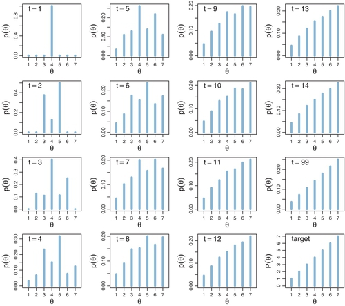
We want to derive the probability of ending up in each position at the next time step. To determine the probabilities of positions for time t = 2, consider the possibilities from the movement process. The process starts with the flip of a fair coin to decide which direction to propose moving. There is a 50% probability of proposing to move right, to θ = 5. By inspecting the target distribution of relative probabilities in the lower-right panel of Figure 7.3, you can see that P (θ=5) > P (θ=4), and therefore, a rightward move is always accepted whenever it is proposed. Thus, at time t = 2, there is a 50% probability of ending up at θ = 5. The panel labeled t = 2 in Figure 7.3 plots this probability as a bar of height 0.5 at θ = 5. The other 50% of the time, the proposed moveis to the left, to θ = 3. By inspecting the target distribution of relative probabilities in the lower-right panel of Figure 7.3, you can see that P(θ =3) = 3, whereas P(θ=4) = 4, and therefore, a leftward move is accepted only 3/4 of the times it is proposed. Hence, at time t = 2, the probability of ending up at θ = 3 is 50%·3/4 = 0.375. The panel labeled t = 2 in Figure 7.3 shows this as a bar of height 0.375 at θ = 3. Finally, if a leftward move is proposed but not accepted, we just stay at θ = 5. The probability of this happening is only 50%·(1 ‒ 3/4) = 0.125.

This process repeats for the next time step. I won't go through the arithmetic details for each value of θ. But it is important to notice that after two proposed moves, i.e., when t = 3, the politician could be at any of the positions θ = 2 through θ = 6, but not yet at θ = 1 or θ = 7, because he could be at most two positions away from where he started.

The probabilities continue to be computed the same way at every time step. You can see that in the early time steps, the probability distribution is not a straight incline like the target distribution. Instead, the probability distribution has a bulge over the starting position. As you can see in Figure 7.3, by time t = 99, the position probability is virtually indistinguishable from the target distribution, at least for this simple distribution. More complex distributions require a longer duration to achieve a good approximation to the target.

The graphs of Figure 7.3 show the probability that the moving politician is at each value of θ. But remember, at any given time step, the politician is at only one particular position, as shown in Figure 7.2. To approximate the target distribution, we let the politician meander around for many time steps while we keep track of where he has been. When we have a long record of where the traveler has been, we can approximate the target probability at each value of θ by simply counting the relative number times that the traveler visited that value.

Here is a summary of our algorithm for moving from one position to another. We are currently at position θ_current. We then propose to move one position right or one position left. The specific proposal is determined by flipping a coin, which can result in 50% heads (move right) or 50% tails (move left). The range of possible proposed moves, and the probability of proposing each, is called the proposal distribution. In the present algorithm, the proposal distribution is very simple: It has only two values with 50-50 probabilities.

Having proposed a move, we then decide whether or not to accept it. The acceptance decision is based on the value of the target distribution at the proposed position, relative to the value of the target distribution at our current position. Specifically, if the target distribution is greater at the proposed position than at our current position, then we definitely accept the proposed move: We always move higher if we can. On the other hand, if the target position is less at the proposed position than at our current position, we accept the move probabilistically: We move to the proposed position with probability p_move = P(θ_proposed)/P(θ_current),where P(θ) is the value of the target distribution at θ. We can combine these two possibilities, of the target distribution being higher or lower at the proposed position than at our current position, into a single expression for the probability of moving to the proposed position:

$p_{\text{move}}=\min \left(\frac{p\left({\theta }_{\text{proposed}}\right)}{p\left({\theta }_{\text{current}}\right)},1\right)$

Notice that Equation 7.1 says that when P(θ_proposed) > P(θ_current),then p_move= 1. Notice also that the target distribution, P(θ), does not need to be normalized, which means it does not need to sum to 1 as a probability distribution must. This is because what matters for our choice is the ratio, P(θ_proposed)/P(θ_current), not the absolute magnitude of P(θ). This property was used in the example of the island-hopping politician: The target distribution was the population of each island, not a normalized probability.

Having proposed a move by sampling from the proposal distribution and having then determined the probability of accepting the move according to Equation 7.1, we then actually accept or reject the proposed move by sampling a value from a uniform distribution over the interval [0,1]. If the sampled value is between 0 and p_move,then we actually make the move. Otherwise, we reject the move and stay at our current position. The whole process repeats at the next time step.

7.2.4 Why we care

Notice what we must be able to do in the random-walk process:

• We must be able to generate a random value from the proposal distribution, to create θ_proposed

• We must be able to evaluate the target distribution at any proposed position, to compute P(θ_proposed)/P(θ_current)

• We must be able to generate a random value from a uniform distribution, to accept or reject the proposal according to p_move.

By being able to do those three things, we are able to do indirectly something we could not necessarily do directly: We can generate random samples from the target distribution. Moreover, we can generate those random samples from the target distribution even when the target distribution is not normalized.

This technique is profoundly useful when the target distribution P(θ) is a posterior proportional to p(D|θ)p(θ). Merely by evaluating p(D|θ)p(θ), without normalizing it by p(D), we can generate random representative values from the posterior distribution. This result is wonderful because the method obviates direct computation of the evidence p(D), which, as you'll recall, is one of the most difficult aspects of Bayesian inference. By using MCMC techniques, we can do Bayesian inference in rich and complex models. It has only been with the development of MCMC algorithms and software that Bayesian inference is applicable to complex data analysis, and it has only been with the production of fast and cheap computer hardware that Bayesian inference is accessible to a wide audience.

7.2.5 Why it works

In this section, I'll explain a bit of the mathematics behind why the algorithm works. Despite the mathematics presented here, however, you will not need to use any of this mathematics for applied data analysis later in the book. The math is presented here only to help you understand why MCMC works. Just as you can drive a car without being able to build an engine from scratch, you can apply MCMC methods without being able to program a Metropolis algorithm from scratch. But it can help you interpret the results of MCMC applications if you know a bit of what is going on “under the hood.”

To get an intuition for why this algorithm works, consider two adjacent positions and the probabilities of moving from one to the other. We'll see that the relative transition probabilities, between adjacent positions, exactly match the relative values of the target distribution. Extrapolate that result across all the positions, and you can see that, in the long run, each position will be visited proportionally to its target value. Now the details: Suppose we are at position θ. The probability of moving to θ + 1, denoted p(θ → θ + 1), is the probability of proposing that move times the probability of accepting it if proposed, which is p(θ → θ + 1) = 0.5 · min (P(θ + 1)/P(θ),1). On the other hand, if we are presently at position θ + 1, the probability of moving to θ is the probability of proposing that move times the probability of accepting it if proposed, which is p(θ + 1 → θ) = 0.5 · min (P(θ)/P(θ + 1),1) The ratio of the transition probabilities is

$\begin{array}{ll}\frac{p(\theta \to \theta +1)}{p(\theta +1\to \theta )}\hfill & =\frac{0.5\min (P(\theta +1)/P(\theta ),1)}{0.5\min (P(\theta )/P(\theta +1),1)}\hfill \\ \hfill & =\{\begin{array}{cc}\frac{1}{P(\theta )/P(\theta +1)}& \mathrm{if}\text{?}P(\theta +1)>P(\theta )\\ \frac{P(\theta +1)/P(\theta )}{1}& if\text{?}P(\theta +1)<P(\theta )\end{array}\hfill \\ \hfill & =\frac{P(\theta +1)}{P(\theta )}\hfill \end{array}$

Equation 7.2 tells us that during transitions back and forth between adjacent positions, the relative probability of the transitions exactly matches the relative values of the target distribution. That might be enough for you to get the intuition that, in the long run, adjacent positions will be visited proportionally to their relative values in the target distribution. If that's true for adjacent positions, then, by extrapolating from one position to the next, it must be true for the whole range of positions.

To make that intuition more defensible, we have to fill in some more details. To do this, I'll use matrix arithmetic. This is the only place in the book where matrix arithmetic appears, so if the details here are unappealing, feel free to skip ahead to the next section (Section 7.3, p. 156). What you'll miss is an explanation of the mathematics underlying Figure 7.3, which depicts the key idea that the target distribution is stable: If the current probability of being in a position matches the target probabilities, then the Metropolis algorithm keeps it that way.

Consider the probability of transitioning from position θ to some other position. The proposal distribution, in the present simple scenario, considers only positions θ + 1 and θ ‒ 1. The probability of moving to position θ ‒ 1 is the probability of proposing that position times the probability of accepting the move if it is proposed: 0.5 min (P(θ − 1)/P(θ),1). The probability of moving to position θ + 1 is the probability of proposing that position times the probability of accepting the move if it is proposed: 0.5 min(P(θ − 1)/P(θ),1). The probability of staying at position θ is simply the complement of those two move-away probabilities: 0.5 [1 − min (P(θ − 1)/P(θ),1)] + 0.5 [1 − min (P(θ + 1)/P(θ),1)].

We can put those transition probabilities into a matrix. Each row of the matrix is a possible current position, and each column of the matrix is a candidate moved-to position. Below is a submatrix from the full transition matrix T , showing rows θ − 2 to θ + 2, and columns θ − 2 to θ + 2:

$\left[\begin{array}{ccccc}\ddots & p\left(\theta -2\to \theta -1\right)& 0& 0& 0\\ \ddots & p\left(\theta -1\to \theta -1\right)& p\left(\theta -1\to \theta \right)& 0& 0\\ 0& p\left(\theta \to \theta -1\right)& p\left(\theta \to \theta \right)& p\left(\theta \to \theta +1\right)& 0\\ 0& 0& p\left(\theta +1\to \theta \right)& p\left(\theta +1\to \theta +1\right)& \ddots \\ 0& 0& 0& p\left(\theta +1\to \theta +1\right)& \ddots \end{array}\right]$

which equals

$\left[\begin{array}{ccccc}\ddots & 0.5\min \left(\frac{p\left(\theta -1\right)}{p\left(\theta -2\right)},1\right)& 0& 0& 0\\ \ddots & \begin{array}{l}0.5\left[1-\min \left(\frac{p\left(\theta -1\right)}{p\left(\theta -2\right)},1\right)\right]\\ +0.5\left[1-\min \left(\frac{p\left(\theta \right)}{p\left(\theta -1\right)},1\right)\right]\end{array}& 0.5\min \left(\frac{p\left(\theta \right)}{p\left(\theta -1\right)},1\right)& 0& 0\\ 0& 0.5\min \left(\frac{p\left(\theta -1\right)}{p\left(\theta \right)},1\right)& \begin{array}{l}0.5\left[1-\min \left(\frac{p\left(\theta -1\right)}{p\left(\theta \right)},1\right)\right]\\ +0.5\left[1-\min \left(\frac{p\left(\theta +1\right)}{p\left(\theta \right)},1\right)\right]\end{array}& 0.5\min \left(\frac{p\left(\theta +1\right)}{p\left(\theta \right)},1\right)& 0\\ 0& 0& 0.5\min \left(\frac{p\left(\theta \right)}{p\left(\theta +1\right)},1\right)& \begin{array}{l}0.5\left[1-\min \left(\frac{p\left(\theta \right)}{p\left(\theta +1\right)},1\right)\right]\\ +0.5\left[1-\min \left(\frac{p\left(\theta +2\right)}{p\left(\theta +1\right)},1\right)\right]\end{array}& \ddots \\ 0& 0& 0& 0.5\min \left(\frac{p\left(\theta +1\right)}{p\left(\theta +2\right)},1\right)& \ddots \end{array}\right]$

The usefulness of putting the transition probabilities into a matrix is that we can then use matrix multiplication to get from any current location to the probability of the next locations. Here's a reminder of how matrix multiplication operates. Consider a matrix T. The value in its rth row and cth column is denoted T_rc. We can multiply the matrix on its left side by a row vector w, which yields another row vector. The cth component of the product wT is ∑_rw_rT_rc. In other words, to compute the cth component of the result, take the row vector w and multiply its components by the corresponding components in the cth column of W, and sum up those component products.³

To use the transition matrix in Equation 7.3, we put the current location probabilities into a row vector, which I will denote w because it indicates where we are. For example, if at the current time, we are definitely in location θ = 4, then w has 1.0 in its θ = 4 component, and zeros everywhere else. To determine the probability of the locations at the next time step, we simply multiply w by T. Here's a key example to think through: When w =[…,0,1,0,…] with a 1 only in the θ position, then wT is simply the row of T corresponding to θ ,because the cth component of wT is ∑_rw_rT_rc=T_θc ,where I'm using the subscript θ to stand for the index that corresponds to value θ.

Matrix multiplication is a very useful procedure for keeping track of position probabilities. At every time step, we just multiply the current position probability vector w by the transition probability matrix T to get the position probabilities for the next time step. We keep multiplying by T, over and over again, to derive the long-run position probabilities. This process is exactly what generated the graphs in Figure 7.3.

Here's the climactic implication: When the vector of position probabilities is the target distribution, it stays that way on the next time step! In other words, the position probabilities are stable at the target distribution. We can actually prove this result without much trouble. Suppose the current position probabilities are the target probabilities, i.e., w=[…,P(θ−1),P(θ),P(θ+1),…]/Z , where Z=∑_θP(θ) is the normalizer for the target distribution. Consider the θ component of wT. We will demonstrate that the θ component of wT is the same as the θ component of w, for any component θ. The θ component of wT is ∑_rw_rT_rθ. Look back at the transition matrix in Equation 7.3, and you can see then that the θ component of wT is

$\begin{array}{ll}\sum _r{w}_r{T}_{r\theta }=\hfill & P(\theta -1)/Z\cdot {0.5}_{\min }(\frac{P(\theta )}{P(\theta -1)},1)\hfill \\ \hfill & +P(\theta )/Z\cdot (0.5)(0.5[1{-}_{\min }(\frac{P(\theta -1)}{P(\theta )},1)]+0.5[1{-}_{\min }(\frac{P(\theta +1)}{P(\theta )},1)])\hfill \\ \hfill & +P(\theta +1)/Z\cdot {0.5}_{\min }(\frac{P(\theta )}{P(\theta +1)},1)\hfill \end{array}$

To simplify that equation, we can consider separately the four cases: Case 1: P(θ) > P(θ − 1) and P(θ) > P(θ + 1); Case2: P(θ) > P(θ − 1) and P(θ) < P(θ + 1); Case 3: P(θ) < P(θ − 1) and P(θ) > P(θ + 1); Case 4: P(θ) < P(θ − 1) and P(θ) < P(θ+1). In each case, Equation 7.4 simplifies to P(θ)/Z. For example, consider Case 1, when P(θ) > P(θ − 1) and P(θ) > P(θ + 1). Equation 7.4 becomes

$\begin{array}{ll}\sum _r{w}_r{T}_{r\theta }\hfill & =P(\theta -1)/Z\text{?}\cdot \text{?}0.5\hfill \\ \hfill & +P(\theta )/Z\cdot (0.5[1-(\frac{P(\theta -1)}{P(\theta )})]+0.5[1-(\frac{P(\theta +1)}{P(\theta )})])\hfill \\ \hfill & +P(\theta +1)/Z\cdot 0.5\hfill \\ \hfill & =0.5\text{?}P(\theta -1)/Z\hfill \\ \hfill & +0.5P(\theta )/Z-0.5P(\theta )/Z\frac{P(\theta -1)}{P(\theta )}+0.5P(\theta )/Z-0.5P(\theta )/Z\frac{P(\theta +1)}{P(\theta )}\hfill \\ \hfill & +0.5P(\theta +1)/Z\hfill \\ \hfill & =P(\theta )/Z\hfill \end{array}$

If you work through the other cases, you'll find that it always reduces to P (θ)/Z. In conclusion, when the θ component starts at P(θ)/Z, it stays at P(θ)/Z.

We have shown that the target distribution is stable under the Metropolis algorithm, for our special case of island hopping. To prove that the Metropolis algorithm realizes the target distribution, we would need to show that the process actually gets us to the target distribution regardless of where we start. Here, I'll settle for intuition: You can see that no matter where you start, the distribution will naturally diffuse and explore other positions. Examples of this were shown in Figures 7.2 and 7.3. It's reasonable to think that the diffusion will settled into some stable state and we've just shown that the target distribution is a stable state. To make the argument complete, we’d have to show that there are no other stable states, and that the target distribution is actually an attractor into which other states flow, rather than a state that is stable if it is ever obtained but impossible to actually attain. This complete argument is far beyond what would be useful for the purposes of this book, but if you're interested you could take a look at the book by Robert and Casella (2004).

7.3.1 Metropolis algorithm applied to Bernoulli likelihood and beta prior

In the scenario of the island-hopping politician, the islands represented candidate parameter values, and the relative populations represented relative posterior probabilities. In the scenario of coin flipping, the parameter θ has values that range on a continuum from zero to one, and the relative posterior probability is computed as likelihood times prior. To apply the Metropolis algorithm, we conceive of the parameter dimension as a dense chain of infinitesimal islands, and we think of the (relative) population of each infinitesimal island as its (relative) posterior probability density. And, instead of the proposed jump being only to immediately adjacent islands, the proposed jump can be to islands farther away from the current island. We need a proposal distribution that will let us visit any parameter value on the continuum. For this purpose, we will use the familiar normal distribution (recall Figure 4.4, p. 83).

We will apply the Metropolis algorithm to the following familiar scenario. We flip a coin N times and observe z heads. We use a Bernoulli likelihood function, p(z, N|θ) = θ^z (1 − θ)^(N−z). We start with a prior p(θ) = beta(θ|a, b). For the proposed jump in the Metropolis algorithm, we will use a normal distribution centered at zero with standard deviation (SD) denoted as σ. We denote the proposed jump as Δθ ~ normal(μ = 0, σ),where the symbol “~” means that the value is randomly sampled from the distribution (cf. Equation 2.2, p. 27). Thus, the proposed jump is usually close to the current position, because the mean jump is zero, but the proposed jump can be positive or negative, with larger magnitudes less likely than smaller magnitudes. Denote the current parameter value as θ_cur and the proposed parameter value as θ_pro = θ_cur + Δθ.

The Metropolis algorithm then proceeds as follows. Start at an arbitrary initial value of θ (in the valid range). This is the current value, denoted θ_cur. Then:

1. $R$andomly generate a proposed jump, Δθ ~ normal(μ = 0, σ) and denote the proposed value of the parameter as θ_pro = θ_cur + Δθ.

2. Compute the probability of moving to the proposed value as Equation 7.1, specifically expressed here as

$\begin{array}{ll}{p}_{move}\hfill & =\min \text{?}(1,\frac{P({\theta }_{pro})}{P({\theta }_{cur})})\text{generic}\text{?}\text{Metropolis}\text{?}\text{form}\hfill \\ \hfill & =\min \text{?}(1,\frac{P\text{?}(D|{\theta }_{pro})p\text{?}({\theta }_{pro})}{P\text{?}(D|{\theta }_{cur})p\text{?}({\theta }_{cur})})P\text{?}\text{is}\text{?}\text{likelihood}\text{?}\text{times}\text{?}\text{prior}\hfill \\ \hfill & \begin{array}{l}=\min \text{?}(1,\frac{Bernoulli\text{?}(z,N|{\theta }_{pro})\text{?}beta\text{?}({\theta }_{pro}|a,b)}{Bernoulli\text{?}(z,N|{\theta }_{cur})\text{?}beta\text{?}({\theta }_{cur}|a,b)})\hfill \\ \text{Bernoulli}\text{?}\text{likelihood}\text{?}\text{and}\text{?}\text{beta}\text{?}\text{prior}\hfill \end{array}\hfill \\ \hfill & \begin{array}{l}=\min \text{?}(1,\frac{{\theta }_{pro}^z{(1-{\theta }_{pro})}^{(N-z)}{\theta }_{pro}^{(a-1)}{(1-{\theta }_{pro})}^{(b-1)}/B(a,b)}{{\theta }_{cur}^z{(1-{\theta }_{cur})}^{(N-z)}{\theta }_{cur}^{(a-1)}{(1-{\theta }_{cur})}^{(b-1)}/B(a,b)})\hfill \\ \text{by}\text{?}\text{Equations}\text{?}\text{6}\text{.2}\text{?}\text{and}\text{?}\text{6}\text{.3}\hfill \end{array}\hfill \end{array}$

If the proposed value θ_pro happens to land outside the permissible bounds of θ ,the prior and/or likelihood is set to zero, hence p_move is zero.

3. Accept the proposed parameter value if a random value sampled from a [0,1] uniform distribution is less than p_move, otherwise reject the proposed parameter value and tally the current value again.

$R$epeat the above steps until it is judged that a sufficiently representative sample has been generated. The judgment of “sufficiently representative” is not trivial and is an issue that will be discussed later in this chapter. For now, the goal is to understand the mechanics of the Metropolis algorithm.

Figure 7.4 shows specific examples of the Metropolis algorithm applied to a case with a beta(θ|1,1) prior, N = 20, and z = 14. There are three columns in Figure 7.4, for three different runs of the Metropolis algorithm using three different values for σ in the proposal distribution. In all three cases, θ was arbitrarily started at 0.01, merely for purposes of illustration.

The middle column of Figure 7.4 uses a moderately sized SD for the proposal distribution, namely σ = 0.2, as indicated in the title of the upper-middle panel where it says “Prpsl.SD = 0.2.” This means that at any step in the chain, for whatever value θ happens to be, the proposed jump is within ±0.2 of θ about 68% of the time (because a normal distribution has about 68% of its mass between ‒1 and +1 SDs). In this case, the proposed jumps are accepted roughly half the time, as indicated in the center panel by the annotation N_acc/N_pro = 0.495, which is the number of accepted proposals divided by the total number of proposals in the chain. This setting of the proposal distribution allows the chain to move around parameter space fairly efficiently. In particular, you can see in the lower-middle panel that the chain moves away quickly from the unrepresentative starting position of θ = 0.01. And, the chain visits a variety of representative values in relatively few steps. That is, the chain is not very clumpy. The upper-middle panel shows a histogram of the chain positions after 50,000 steps. The histogram looks smooth and is an accurate approximation of the true underlying posterior distribution, which we know in this case is a beta(θ|15,7) distribution (cf. Figure 7.1, p. 146). Although the chain is not very clumpy and yields a smooth-looking histogram, it does have some clumpiness because each step is linked to the location of the previous step, and about half the steps don't change at all. Thus, there are not 50,000 independent representative values of the posterior distribution in the chain. If we take into account the clumpiness, then the so-called “effective size” of the chain is less, as indicated in the title of upper-middle panel where it says “Eff.Sz. = 11723.9.” This is the equivalent number of values if they were sampled independently of each other. The technical meaning of effective size will be discussed later in the chapter.

The left column of Figure 7.4 uses a relatively small proposal SD, namely σ = 0.02, as indicated in the title of the upper-left panel where it says “Prpsl.SD = 0.02.” You can see that successive steps in the chain make small moves because the proposed jumps are small. In particular, in the lower-left panel you can see that it takes many steps for the chain to move away from the unrepresentative starting position of θ = 0.01. The chain explores values only very gradually, producing a snake-like chain that lingers around particular values, thereby producing a form of clumpiness. In the long run, the chain will explore the posterior distribution thoroughly and produce a good representation, but it will require a very long chain. The title of the upper-left panel indicates that the effective size of this 50,000 step chain is only 468.9.

The right column of Figure 7.4 uses a relatively large proposal SD, namely σ = 2, as indicated in the title of the upper-left panel where it says “Prpsl.SD = 2.” The proposed jumps are often far away from the bulk of the posterior distribution, and therefore, the proposals are often rejected and the chain stays at one value for many steps. The process accepts new values only occasionally, producing a very clumpy chain. In the long run, the chain will explore the posterior distribution thoroughly and produce a good representation, but it will require a very long chain. The title of the upper-right panel indicates that the effective size of this 50,000 step chain is only 2113.4.

$R$egardless of the which proposal distribution in Figure 7.4 is used, the Metropolis algorithm will eventually produce an accurate representation of the posterior distribution, as is suggested by the histograms in the upper row of Figure 7.4. What differs is the efficiency of achieving a good approximation. The moderate proposal distribution will achieve a good approximation in fewer steps than either of the extreme proposal distributions. Later in the chapter, we will discuss criteria for deciding that a chain has produced a sufficiently good approximation, but for now suppose that our goal is to achieve an effective size of 10,000. The proposal distribution in the middle column of Figure 7.4 has achieved this goal. For the proposal distribution in the left column of Figure 7.4, we would need to run the chain more than 20 times longer because the effective size is less than 1/20th of the desired size. Sophisticated implementations of the Metropolis algorithm have an automatic preliminary phase that adjusts the width of the proposal distribution so that the chain moves relatively efficiently. A typical way to do this is to adjust the proposal distribution so that the acceptance ratio is a middling value such as 0.5. The steps in the adaptive phase are not used to represent the posterior distribution.

7.3.2 Summary of Metropolis algorithm

In this section, I recapitulate the main ideas of the Metropolis algorithm and explicitly point out the analogy between the island-hopping politician and the θ-hopping coin bias.

The motivation for methods like the Metropolis algorithm is that they provide a high-resolution picture of the posterior distribution, even though in complex models we cannot explicitly solve the mathematical integral in Bayes’ rule. The idea is that we get a handle on the posterior distribution by generating a large sample of representative values. The larger the sample, the more accurate is our approximation. As emphasized previously, this is a sample of representative credible parameter values from the posterior distribution; it is not a resampling of data (there is a fixed data set).

The cleverness of the method is that representative parameter values can be randomly sampled from complicated posterior distributions without solving the integral in Bayes’ rule, and by using only simple proposal distributions for which efficient random number generators already exist. All we need to decide whether to accept a proposed parameter value is the mathematical formulas for the likelihood function and prior distribution, and these formulas can be directly evaluated from their definitions.

We have seen two examples of the Metropolis algorithm in action. One was the island-hopping politician in Figure 7.2. The other was the θ-hopping coin bias in Figure 7.4. The example of the island-hopping politician was presented to demonstrate the Metropolis algorithm in its most simple form. The application involved only a finite space of discrete parameter values (i.e., the islands), the simplest possible proposal distribution (i.e., a single step right or left), and a target distribution that was directly evaluated (i.e., the relative population of the island) without any reference to mathematical formulas for likelihood functions and prior distributions. The simple forms of the discrete space and proposal distribution also allowed us to explore some of the basic mathematics of transition probabilities, to get some sense of why the Metropolis algorithm works.

The example of the θ -hopping coin bias in Figure 7.4 used the Metropolis algorithm in a more realistic setting. Instead of a finite space of discrete parameter values, there was a continuum of possible parameter values across the interval from zero to one. This is like an infinite string of adjacent infinitesimal islands. Instead of a proposal distribution that could only go a single step left or right, the normal proposal distribution could jump anywhere on the continuum, but it favored nearby values as governed by the SD of its bell shape. And, instead of a simple “relative population” at each parameter value, the target distribution was the relative density of the posterior distribution, computed by evaluating the likelihood function times the prior density.

7.4.1 Prior, likelihood and posterior for two biases

We are considering situations in which there are two underlying biases, namely θ₁ and θ₂, for the two coins. We are trying to determine what we should believe about these biases after we have observed some data from the two coins. $R$ecall that I am using the term “bias” as the name of the parameter θ, and not to indicate that the value of θ deviates from 0.5. The colloquial meaning of bias, as unfair, might also sneak into my writing from time to time. Thus, a colloquially “unbiased” coin technically “has a bias of 0.5.”

To estimate the biases of the coins in a Bayesian framework, we must first specify what we believe about the biases without the data. Our prior beliefs are about combinations of parameter values. To specify a prior belief, we must specify the credibility, p(θ₁,θ₂),for every combination θ₁,θ₂. If we were to make a graph of p(θ₁,θ₂), it would be three dimensional, with θ₁ and θ₂ on the two horizontal axes, and p(θ₁,on the vertical axis. Because the credibilities form a probability density function, their integral across the parameter space must be one: ${\displaystyle \iint \text{d}{\theta }_1\text{d}{\theta }_{2}p\left({\theta }_1,{\theta }_2\right)=1}$.

For simplicity in these examples, we will assume that our beliefs about θ₁ are independent of our beliefs about θ₂. For example, if I have a coin from Canada and a coin from India, my belief about bias in the coin from Canada could be completely separate from my belief about bias in the coin from India. Independence of attributes was discussed in Section 4.4.2, p. 92. Mathematically, independence means that p(θ₁,θ₂)= p(θ₁)p(θ₂) for every value of θ₁ and θ₂,where p(θ₁) and p(θ₂) are the marginal belief distributions. When beliefs about two parameters are independent, the mathematical manipulations can be greatly simplified. Beliefs about the two parameters do not need to be independent, however. For example, perhaps I believe that coins are minted in similar ways across countries, and so if a Canadian coin is biased (i.e., has a θ value different than 0.5), then an Indian coin should be similarly biased. At the extreme, if I believe that θ₁ always exactly equals θ₂, then the two parameter values are completely dependent upon each other. Dependence does not imply direct causal relationship, it merely implies that knowing the value of one parameter constrains beliefs about the value of the other parameter.

Along with the prior beliefs, we have some observed data. We assume that the flips within a coin are independent of each other and that the flips across coins are independent of each other. The veracity of this assumption depends on exactly how the observations are actually made, but, in properly designed experiments, we have reasons to trust this assumption. Notice that we will always assume independence of data within and across groups, regardless of whether we assume independence in our beliefs about the biases in the groups. Formally, the assumption of independence in the data means the following. Denote the result of a flip of coin 1 as y₁, where the result can be y₁ = 1(heads) or y₁ = 0 (tails). Similarly, the result of a flip of coin 2 is denoted y2. Independence of the data across the two coins means that the data from coin 1 depend only on the bias in coin 1, and the data from coin 2 depend only on the bias in coin 2, which can be expressed formally as p(y₁|θ₁θ₂),= p(y₁|θ₁) and p(y₂|θ₁,θ₂=p(y₂|θ₂)

From one coin we observe the data D₁ consisting of z₁ heads out of N₁ flips, and from the other coin we observe the data D₂ consisting of z₂ heads out of N₂ flips. In other words, $z_1={{\sum }^{\text{}}}_{i=1}^{N_1}y1i$, where y1i denotes the ith flip of the first coin. Notice that z₁ ∈ {0,…,N₁} and z₂ ∈ {0,…, N₂}. We denote the whole set of data as D ={z₁, N₁, z₂, N₂}. Because of independence of sampled flips, the probability of D is the product of the Bernoulli distribution functions for the individual flips:

$\begin{array}{ll}p(D|{\theta }_1,{\theta }_2)\hfill & =\prod _{y_{1i}\in D_1}p(y_{1i}|{\theta }_1,{\theta }_2)\prod _{y_{2j}\in D_2}p(y_{2j}|{\theta }_1,{\theta }_2)\hfill \\ \hfill & =\prod _{y_{1i}\in D_1}{\theta }_1^{y_{1i}}{(1-{\theta }_1)}^{(1-y_{1i})}\prod _{y_{2i}\in D_2}{\theta }_2^{y_{2i}}{(1-{\theta }_2)}^{(1-y_{2j})}\hfill \\ \hfill & ={\theta }_1^{z_1}{(1-{\theta }_1)}^{(N_1-z_1)}{\theta }_2^{z_2}{(1-{\theta }_2)}^{(N_2-z_2)}\hfill \end{array}$

The posterior distribution of our beliefs about the underlying bias is derived in the usual way by applying Bayes’ rule, but now the functions involve two parameters:

$\begin{array}{l}p\left({\theta }_1,{\theta }_2|D\right)=p\left(D|{\theta }_1,{\theta }_2\right)p\left({\theta }_1,{\theta }_2\right)/p\left(D\right)\\ =p\left(D|{\theta }_1,{\theta }_2\right)p\left({\theta }_1,{\theta }_2\right)/{\displaystyle \iint \text{d}{\theta }_{\text{1}}\text{d}{\theta }_{\text{2}p}\left(D|{\theta }_1,{\theta }_2\right)p\left({\theta }_1,{\theta }_2\right)}\end{array}$

$R$emember, as always in the expression of Bayes’ rule, the θ_j's in left side of the equation and in the numerator of the right side are referring to specific values of θ_j, but the θ_j's in the integral in the denominator range over all possible values of θ_j.

What has just been described in the previous few paragraphs is the general Bayesian framework for making inferences about two biases when the likelihood function consists of independent Bernoulli distributions. What we have to do next is specify a particular mathematical form for the prior distribution. We will work through the mathematics of a particular case for two reasons: First, it will allow us to explore graphical displays of two-dimensional parameter spaces, which will inform our intuitions about Bayes’ rule and sampling from the posterior distribution. Second, the mathematics will set the stage for a specific example of Gibbs sampling. Later in the book when we do applied Bayesian analysis, we will not be doing any of this sort of mathematics. We are doing the math now, for simple cases, to understand how the methods work so we can properly interpret their outputs in realistically complex cases.

7.4.2 The posterior via exact formal analysis

Suppose we want to pursue a solution to Bayes’ rule, in Equation 7.6 above, using formal analysis. What sort of prior probability function would make the analysis especially tractable? Perhaps you can guess the answer by recalling the discussion of Chapter 6. We learned there that the beta distribution is conjugate to the Bernoulli likelihood function. This suggests that a product of beta distributions would be conjugate to a product of Bernoulli functions.

This suggestion turns out to be true. We pursue the same logic as was used for Equation 6.8 (p. 132). First, recall that a beta distribution has the form beta(θ|a,b)=θ^(a−1)(1−θ)^(b−1)/B(a,b), where B(a, b) is the beta normalizing function, which by definition is $B(a,b)={\displaystyle {\int }_0^{1}d\theta \text{?}{\theta }^{(a-1)}{(1-\theta )}^{(b-1)}}$. We assume a beta(θ₁|a₁, b₁) prior on θ₁, and an independent beta(θ₂|a₂, b₂) prior on θ₂, so that p(θ₁,θ₂) = beta(θ₁|a₁, b₁) · beta(θ₂|a₂, b₂). Then:

$\begin{array}{ll}p({\theta }_1,{\theta }_2|D)\hfill & =p(D|{\theta }_1,{\theta }_2)p({\theta }_1,{\theta }_2)/p(D)\text{general}\text{?}\text{form}\text{?}\text{of}\text{?}\text{Bayes'}\text{?}\text{rule}\hfill \\ \hfill & \begin{array}{l}={\theta }_1^{z_1}{(1-{\theta }_1)}^{(N_1-z_1)}{\theta }_2^{z_2}{(1-{\theta }_2)}^{(N_2-z_2)}p({\theta }_1,{\theta }_2)/p(D)\hfill \\ \text{Bernoulli}\text{?}\text{likelihood}\text{?}\text{from}\text{?}\text{Equation}\text{?}7.5\hfill \end{array}\hfill \\ \hfill & \begin{array}{l}=\frac{{\theta }_1^{z_1}{(1-{\theta }_1)}^{(N_1-z_1)}{\theta }_2^{z_2}{(1-{\theta }_2)}^{(N_2-z_2)}{\theta }_1^{(a_1-1)}{(1-{\theta }_1)}^{(b_1-1)}{\theta }_2^{(a_2-1)}{(1-{\theta }_2)}^{(b_2-1)}}{p(D)B(a_1,b_1)B(a_2,b_2)}\hfill \\ \text{independent}\text{?}\text{beta}\text{?}\text{prior}\hfill \end{array}\hfill \\ \hfill & =\frac{{\theta }_1^{(z_1+a_1-1)}{(1-{\theta }_1)}^{(N_1-z_1+b_1-1)}{\theta }_2^{(z_2+a_2-1)}{(1-{\theta }_2)}^{(N_2-z_2+b_2-1)}}{p(D)B(a_1,b_1)B(a_2,b_2)}\hfill \end{array}$

We know that the left side of Equation 7.7 must be a probability density function, and we see that the numerator of the right side has the form of a product of beta distributions, namely beta(θ₁|z₁ +a₁, N₁ − z₁ +b₁) times beta(θ₂|z₂ + a₂, N₂ − z₂ + b₂). Therefore, the denominator of Equation 7.7 must be the corresponding normalizer for the product of beta distributions:⁵

$p\left(D\right)B\left(a_1,b_1\right)B\left(a_2,b_2\right)=B\left(z_1+a_1,N_1-z_1+b_1\right)B\left(z_2+a_2,N_2-z_2+b_2\right)$

Recapitulation: When the prior is a product of independent beta distributions, the posterior is also a product of independent beta distributions, with each beta obeying the update rule we derived in Chapter 6. Explicitly, if the prior is beta(θ₁|a₁, b₁)· beta(θ₂|a₂, b₂), and the data are z₁, N₁, z₂, N₂, then the posterior is beta(θ₁|z₁+a₁, N₁ − z₁ + b₁) · beta(θ₂|z₂ + a₂,N₂ − z₂ + b₂).

One way of understanding the posterior distribution is to visualize it. We want to plot the probability densities as a function of two parameters, θ₁ and θ₂. One way todo this is by placing the two parameters, θ₁ and θ₂, on two horizontal axes, and placing the probability density, p(θ₁,θ₂), on a vertical axis. The surface can then be displayed in a picture as if it were a landscape viewed in perspective. Alternatively, we can place the two parameter axes flat on the drawing plane and indicate the probability density with level contours, such that any one contour marks points that have the same specific level. An example of these plots is described next.

Figure 7.5 shows graphs for an example of Bayesian updating from Equation 7.6. In this example, the prior begins with mild beliefs that each bias is about 0.50, using a beta(θ|2, 2) distribution for both biases. The upper panels show a perspective plot and a contour plot for the prior distribution. Notice that it is gently peaked at the center of the parameter space, which reflects the prior belief that the two biases are around 0.5, but without much certainty. The perspective plot shows vertical slices of the prior density parallel to θ₁ and θ₂. Consider slices parallel to the θ₁ axis, with different slices at different values of θ₂. The profile of the density on every slice has the same shape, with merely different heights. In particular, at every level of θ₂, the profile of the slice along θ₁ is a beta(θ₁|2,2) shape, with merely an overall height that depends on the level of θ₂. When the shape of the profile on the slices does not change, as exemplified here, then the joint distribution is constructed from the product of independent marginal distributions.

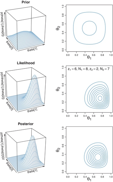
The contour plot in the upper-right panel of Figure 7.5 shows the same distribution as the upper-left panel. Instead of showing vertical slices through the distribution, the contour plot shows horizontal slices. Each contour corresponds to a slice at a particular height. Contour plots can be challenging to interpret because it is not immediately obvious what the heights of the contours are, or even whether two adjacent contours belong to different heights. Contours can be labeled with numerical values to indicate their heights, but then the plot can become very cluttered. Therefore, if the goal is a quick intuition about the general layout of the distribution, then a perspective plot is preferred over a contour plot. If the goal is instead a more detailed visual determination of the parameter values for a particular peak in the distribution, then a contour plot may be preferred.

The middle row of Figure 7.5 shows the likelihood functions for the specific data displayed in the panels. The plots show the likelihood for each possible combination of θ₁ and θ₂ . Notice that the likelihood is maximized at θ values that match the proportions of heads in the data.

The resulting posterior distribution is shown in the lowest row of Figure 7.5. At each point in the θ₁, θ₂ parameter space, the posterior is the product of the prior and likelihood values at that point, divided by the normalizer, p(D).

Summary: This section provided a graphical display of a prior, likelihood, and posterior on a two-parameter space, in Figure 7.5. In this section, we emphasized the use ofmathematical forms, with priors that are conjugate to the likelihood. The particular mathematical form, involving beta distributions, will be used again in a subsequent section that introduces Gibbs sampling, and that is another motivation for including the mathematical formulation of this section. Before getting to Gibbs sampling, however, we first apply the Metropolis algorithm to this two-parameter situation. We will see later that Gibbs sampling generates a posterior sample more efficiently than the Metropolis algorithm.

7.4.3 The posterior via the Metropolis algorithm

Although we have already solved the present example with exact mathematical analysis, we will apply the Metropolis algorithm to expand our understanding of the algorithm for a two-parameter case and subsequently to compare the Metropolis algorithm with Gibbs sampling. $R$ecall that the Metropolis algorithm is a random walk through the parameter space that starts at some arbitrary point. We propose a jump to a new point in parameter space, with the proposed jump randomly generated from a proposal distribution from which it is easy to generate values. For our present purposes, the proposal distribution is a bivariate normal. You can visualize a bivariate normal distribution by imagining a one-dimensional normal (as in Figure 4.4, p. 83), sticking a pin down vertically through its peak, and spinning it around the pin, to form a bell-shaped surface. The use of a bivariate normal proposal distribution implies that the proposed jumps will usually be near the current position. Notice that proposed jumps can be in any direction in parameter space relative to the current position.⁶ The proposed jump is definitely accepted if the posterior is taller (more dense) at the proposed position than at the current position, and the proposed jump is probabilistically accepted if the posterior is shorter (less dense) at the proposed position than at the current position. If the proposed jump is rejected, the current position is counted again. Notice that a position in parameter space represents a combination of jointly credible parameter values, 〈θ₁,θ₂〉.

Figure 7.6 shows the Metropolis algorithm applied to the case of Figure 7.5 (p. 167), so that you can directly compare the results of the Metropolis algorithm with the results of formal analysis and grid approximation. By comparing with the contour plot in the lower-right panel of Figure 7.5 (p. 167), you can see that the points do indeed appear to explore the bulk of the posterior distribution. The sampled points in Figure 7.6 are connected by lines so that you can get a sense of the trajectory taken by the random walk. But the ultimate estimates regarding the posterior distribution do not care about the sequence in which the sampled points appeared, and the trajectory is irrelevant to anything but your understanding of the Metropolis algorithm.

The two panels of Figure 7.6 show results from using two different widths for the proposal distribution. The left panel shows results from a relatively narrow proposal distribution, that had a standard deviation of only 0.02. You can see that there were only tiny changes from one step to the next. Visually, the random walk looks like a clumpy strand that gradually winds through the parameter space. Because the proposed jumps were so small, the proposals were usually accepted, but each jump yielded relatively little new information and consequently the effective sample size (ESS) of the chain is very small, as annotated at the top of the panel.

The right panel of Figure 7.6 shows results from using a moderate width for the proposal distribution, with a SD of 0.2. The jumps from one position to the next are larger than the previous example, and the random walk explores the posterior distribution more efficiently than the previous example. The ESS of the chain is much larger than before. But the ESS of the chain is still far less than the number of proposed jumps, because many of the proposed jumps were rejected, and even when accepted, the jumps tended to be near the previous step in the chain.

In the limit of infinite random walks, the Metropolis algorithm yields arbitrarily accurate representations of the underlying posterior distribution. The left and right panels of Figure 7.6 would eventually converge to an identical and highly accurate approximation to the posterior distribution. But in the real world of finite random walks, we care about how efficiently the algorithm generates an accurate representative sample. We prefer to use the proposal distribution from the right panel of Figure 7.6 because it will, typically, produce a more accurate approximation of the posterior than the proposal distribution from left panel, for the same number of proposed jumps.

7.4.4 Gibbs sampling

The Metropolis algorithm is very general and broadly applicable. One problem with it, however, is that the proposal distribution must be properly tuned to the posterior distribution if the algorithm is to work well. If the proposal distribution is too narrow or too broad, a large proportion of proposed jumps will be rejected and the trajectory will get bogged down in a localized region of the parameter space. Even at its most efficient, the effective size of the chain is far less than the number of proposed jumps. It would be nice, therefore, if we had another method of sample generation that was more efficient. Gibbs sampling is one such method.

Gibbs sampling was introduced by Geman and Geman (1984), who were studying how computer vision systems could infer properties of an image from its pixelated camera input. The method is named after the physicist Josiah Willard Gibbs (1839-1903), who studied statistical mechanics and thermodynamics. Gibbs sampling can be especially useful for hierarchical models, which we explore in Chapter 9. It turns out that Gibbs sampling is a special case of the Metropolis-Hastings algorithm, which is a generalized form of the Metropolis algorithm, as will be briefly discussed later. An influential article by Gelfand and Smith (1990) introduced Gibbs sampling to the statistical community; a brief review is provided by Gelfand (2000), and interesting details of the history of MCMC can be found in the book by McGrayne (2011).

The procedure for Gibbs sampling is a type of random walk through parameter space, like the Metropolis algorithm. The walk starts at some arbitrary point, and at each point in the walk, the next step depends only on the current position, and on no previous positions. What is different about Gibbs sampling, relative to the Metropolis algorithm, is how each step is taken. At each point in the walk, one of the component parameters is selected. The component parameter could be selected at random, but typically the parameters are cycled through, in order: θ₁,θ₂,θ₃,…, θ₁,θ₂,θ₃,…. The reason that parameters are cycled rather than selected randomly is that for complex models with many dozens or hundreds of parameters, it would take too many steps to visit every parameter by random chance alone, even though they would be visited about equally often in the long run. Suppose that parameter θ_i has been selected. Gibbs sampling then chooses a new value for that parameter by generating a random value directly from the conditional probability distribution p(θ_i|{θ_j≠i}, D. The new value for θ_i, combined with the unchanged values of θ_j≠i, constitutes the new position in the random walk. The process then repeats: Select a component parameter and select a new value for that parameter from its conditional posterior distribution.

Figure 7.7 illustrates this process for a two-parameter example. In the first step, we want to select a new value for θ₁. We conditionalize on the values of all the other parameters, θ_j≠1 , from the previous step in the chain. In this example, there is only one other parameter, namely θ₂. The upper panel of Figure 7.7 shows a slice through the joint distribution at the current value of θ₂. The heavy curve is the posterior distribution conditional on this value of θ₂, denoted p(θ₁|{θ_j≠1}, D, which is p(θ₁|θ₂, D) in this case because there is only one other parameter. If the mathematical form of the conditional distribution is appropriate, a computer can directly generate a random value of θ₁. Having thereby generated a new value for θ₁, we then conditionalize on it and determine the conditional distribution of the next parameter, θ₂, as shown in the lower panel of Figure 7.7. The conditional distribution is denoted formally as p(θ₂|{θ_j≠2}, D, which equals p(θ₂|θ₁,D) in this case of only two parameters. If the mathematical form is convenient, our computer can directly generate a random value of θ₂ from the conditional distribution. We then conditionalize on the new value θ₂, and the cycle repeats.

Gibbs sampling can be thought of as just a special case of the Metropolis algorithm, in which the proposal distribution depends on the location in parameter space and the component parameter selected. At any point, a component parameter is selected, and then the proposal distribution for that parameter's next value is the conditional posterior probability of that parameter. Because the proposal distribution exactly mirrors the posterior probability for that parameter, the proposed move is always accepted. A rigorous proof of this idea requires development of a generalized form of the Metropolis algorithm, called the Metropolis-Hastings algorithm (Hastings, 1970). A technical overview of the relation is provided by Chib and Greenberg (1995), and an accessible mathematical tutorial is given by Bolstad (2009).

Gibbs sampling is especially useful when the complete joint posterior, p({θ_i}|D), cannot be analytically determined and cannot be directly sampled, but all the conditional distributions, p(θ_i|{θ_j≠i}, D, can be determined and directly sampled. We will not encounter such a situation until later in the book, but the process of Gibbs sampling can be illustrated now for a simpler situation.

We continue now with estimating two coin biases, θ₁ and θ₂, when assuming that the prior belief distribution is a product of beta distributions. The posterior distribution is again a product of beta distributions, as was derived in Equation 7.7 (p. 165). This joint posterior is easily dealt with directly, and so there is no real need to apply Gibbs sampling, but we will go ahead and do Gibbs sampling of this posterior distribution for purposes of illustration and comparison with other methods.

To accomplish Gibbs sampling, we must determine the conditional posterior distribution for each parameter. By definition of conditional probability,

$\begin{array}{l}\begin{array}{cc}p({\theta }_1|{\theta }_2,D)& =p({\theta }_1,{\theta }_2|D)/p({\theta }_2|D)\text{conditional is joint divided by marginal}\\ & \begin{array}{c}\\ =p({\theta }_1,{\theta }_2|D)/{\int }^{\text{}}d{\theta }_{1}p({\theta }_1,{\theta }_2|D)\text{?}\text{?}\text{marginal is integral of joint}\end{array}\end{array}\\ \end{array}$

For our current application, the joint posterior is a product of beta distributions, as was derived in Equation 7.7, p. 165. Therefore, substituting into the equation above, we have

$\begin{array}{cc}p\left({\theta }_1|{\theta }_2,\text{?}D\right)& =p\left({\theta }_1,\text{?}{\theta }_2|D\right)/{\displaystyle \int \text{d}{\theta }_{1}p\left({\theta }_1,\text{?}{\theta }_2|D\right)}\hfill \\ & =\frac{\text{beta}\left({\theta }_1|z_1+a_1,\text{?}{N}_1-z_1+b_1\right)\text{?}\text{beta}\left({\theta }_2|z_2+a_2,\text{?}{N}_2-z_2+b_2\right)}{{\displaystyle \int \text{d}{\theta }_1\text{?}\text{beta}\left({\theta }_1|z_1+a_1,\text{?}{N}_1-z_1+b_1\right)\text{?}\text{beta}\left({\theta }_2|z_2+a_2,\text{?}{N}_2-z_2+b_2\right)}}\hfill \\ & =\frac{\text{beta}\left({\theta }_1|z_1+a_1,\text{?}{N}_1-z_1+b_1\right)\text{?}\text{beta}\left({\theta }_2|z_2+a_2,\text{?}{N}_2-z_2+b_2\right)}{\begin{array}{c}\text{beta}\left({\theta }_2|z_2+a_2,\text{?}{N}_2-z_2+b_2\right)\text{?}{\displaystyle \int \text{d}{\theta }_{\text{1}}\text{?}\text{beta}\left({\theta }_1|z_1+a_1,\text{?}{N}_1-z_1+b_1\right)}\\ \text{?}\text{?}\text{because}\text{?}\text{beta}\left({\theta }_2|\dots \right)\text{is}\text{?}\text{constant}\text{?}\text{w}\text{.r}\text{.t}\text{.}\text{?}{\theta }_{\text{1}}\end{array}}\hfill \\ & =\frac{\text{beta}\left({\theta }_1|z_1+a_1,\text{?}{N}_1-z_1+b_1\right)\text{?}\text{beta}\left({\theta }_2|z_2+a_2,\text{?}{N}_2-z_2+b_2\right)}{\begin{array}{c}\text{beta}\left({\theta }_2|z_2+a_2,\text{?}{N}_2-z_2+b_2\right)\\ \text{?}\text{?}\text{because}\text{?}\text{integral}\text{?}\text{of}\text{?}\text{prob}\text{.}\text{?}\text{distrib}\text{.}\text{?}\text{must}\text{?}\text{be}\text{?}\text{1}\end{array}}\hfill \\ & =\text{beta}\left({\theta }_1|z_1+a_1,\text{?}{N}_1-z_1+b_1\right)\hfill \end{array}$

From these considerations, you can also see that the other conditional posterior probability is p(θ₂|θ₁, D) = beta(θ₂|z₂+a₂, N₂−Z₂+b₂). We have just derived what may have already been intuitively clear: Because the posterior is a product of independent beta distributions, it makes sense that p(θ₁|θ₂, D) = p(θ₁|D). Nevertheless, the derivation illustrates the sort of analytical procedure that is needed in general. In general, the posterior distribution will not be a product of independent marginal distributions as in this simple case. Instead, the formula for p(θ_i|θ_j≠i, D) will typically involve the values of θ_j≠i.

The conditional distributions just derived were displayed graphically in Figure 7.7. The upper panel shows a slice conditional on θ₂, and the heavy curve illustrates p(θ₁|θ₂, D) which isbeta(θ₁|z₁+a₁, N₁−Z₁+b₁). The lower panel shows a slice conditional on θ₁,and theheavy curveillustrates p(θ₂|θ₁, D), which is beta(θ₂|z₂+a₂, N₂−Z₂+b₂).

Having successfully derived the conditional posterior probability distributions, we now figure out whether we can directly sample from them. In this case, the answer is yes, we can, because the conditional probabilities are beta distributions, and our computer software comes prepackaged with generators of random beta values.

Figure 7.8 shows the result of applying Gibbs sampling to this scenario. The left panel shows every step, changing one parameter at a time. Notice that each step in the random walk is parallel to a parameter axis, because each step changes only one component parameter. You can also see that at each point, the walk direction changes to the other parameter, rather than doubling back on itself or continuing in the same direction. This is because the walk cycled through the component parameters, θ₁, θ₂,θ₁, θ₂,θ₁, θ₂, rather than selecting them randomly at each step.

The right panel of Figure 7.8 only shows the steps after each complete cycle through the parameters. It is the same chain as in the left panel, only with the intermediate steps not shown. Both the left and the right panels are representative samples from the posterior distribution, and they would converge to the same continuous distribution in the limit of an infinitely long chain. The software we will use later in the book (called JAGS) records only complete cycles, not intermediate single-parameter steps.

If you compare the results of Gibbs sampling in Figure 7.8 with the results of the Metropolis algorithm in Figure 7.6 (p. 169), you will see that the points produced by Gibbs sampling and the Metropolis algorithm look similar in where they fall, if not in the trajectory of the walk that produces them. In fact, in the infinitely long run, the Gibbs and Metropolis methods converge to the same distribution. What differs is the efficiency of getting to any desired degree of approximation accuracy in a finite run. Notice that the effective size of the Gibbs sampler, displayed in the panel annotations of Figure 7.8, is much greater than the effective size of the Metropolis algorithm displayed in Figure 7.6. (The right panel of Figure 7.8 shows that the effective size is the same as the number of complete cycles of the Gibbs sampler in this case, but this is not generally true and happens here because the conditional distributions are independent of each other.)

By helping us visualize how Gibbs sampling works, Figure 7.8 also helps us understand better why it works. Imagine that instead of changing the component parameter at every step, we linger a while on a component. Suppose, for example, that we have a fixed value of θ₁, and we keep generating new random values of θ₂ for many steps. In terms of Figure 7.8, this amounts to lingering on a vertical slice of the parameter space, lined up over the fixed value of θ₁. As we continue sampling within that slice, we build up a good representation of the posterior distribution for that value of θ₁. Now we jump to a different value of θ₁, and again linger a while at the new value, filling in a new vertical slice of the posterior. If we do that enough, we will have many vertical slices, each representing the posterior distribution along that slice. We can use those vertical slices to represent the posterior, if we have also lingered in each slice proportionally to the posterior probability of being in that slice! Not all values of θ₁ are equally likely in the posterior, so we visit vertical slices according to the conditional probability of θ₁. Gibbs sampling carries out this process, but lingers for only one step before jumping to anewslice.

So far, I have emphasized the advantages of Gibbs sampling over the Metropolis algorithm, namely, that there is no need to tune a proposal distribution and no inefficiency of rejected proposals. I also mentioned restrictions: We must be able to derive the conditional probabilities of each parameter on the others and be able to generate random samples from those conditional probability distributions.

But there is one other disadvantage of Gibbs sampling. Because it only changes one parameter value at a time, its progress can be stalled by highly correlated parameters. We will encounter applications later in which credible combinations of parameter values can be very strongly correlated; see, for example, the correlation of slope and intercept parameters in Figure 17.3, p. 481. Here I hope merely to plant the seeds of an intuition for later development. Imagine a posterior distribution over two parameters. Its shape is a narrow ridge along the diagonal of the parameter space, and you are inside, within, this narrow ridge, like being inside a long-narrow hallway that runs diagonally to the parameter axes. Now imagine doing Gibbs sampling from this posterior. You are in the hallway, and you are contemplating a step along a parameter axis. Because the hallway is narrow and diagonal, a step along a parameter axis quickly encounters a wall, and your step size must be small. This is true no matter which parameter axis you face along. Therefore, you can take only small steps and only very gradually explore the length of the diagonal hallway. On the other hand, if you were stepping according to a Metropolis sampler, whereby your proposal distribution included changes of both parameters at once, then you could jump in the diagonal direction and quickly explore the length of the hallway.

7.4.5 Is there a difference between biases?

Until this point, we have focused on the mechanics of Gibbs sampling (and the Metropolis algorithm) without answering the question, How different are the biases of the two coins? Fortunately, the representative sample from the joint posterior distribution gives us an answer. Notice that every step in the chain (either from Gibbs or Metropolis) is a combination of θ₁ and θ₂ values that are jointly credible. Therefore, at each step in the chain, a credible difference is θ₁ − θ₂. Across the full chain, we have a large representative sample of credible differences. (We cannot get a sense of the difference of parameters merely by looking at the marginal distributions of those parameters; see Section 12.1.2.1, p. 340.)

Figure 7.9 shows histograms of θ₁ − θ₂ from the posterior distribution, generated by each of the chains in Figures 7.6 and 7.8. In the limit of an infinite chain, they would all converge to the same true underlying posterior distribution, but any finite chain is an approximation. In principle, on average, the results from a chain with larger effective size should be more accurate than a smaller effective size, although the smaller might get lucky and happen to be more accurate on a given random walk. In this case, therefore, the results from the Gibbs sampling are probably more accurate than the results from the Metropolis algorithm.

Figure 7.9 reveals that a difference of zero is clearly among the 95% most credible differences (i.e., within the 95% HDI), and we would not want to declare that there is a difference. The Bayesian posterior gives complete information about credible differences and indicates that there is a suggestion of difference, but our uncertainty is large because the amount of data is small. Notice that the decision rule is a separate process from Bayes’ rule, and the result of a decision rule leaves behind most of the posterior information. See Section 12.1.1, p. 336, for complete discussion of HDI and decisions.

7.4.6 Terminology: MCMC

Assessing the properties of a target distribution by generating representative random values is a case of a Monte Carlo simulation. Any simulation that samples a lot of random values from a distribution is called a Monte Carlo simulation, named after the dice and spinners and shufflings of the famous casino locale. The appellation “Monte Carlo” is attributed (Eckhardt, 1987) to the mathematicians Stanislaw Ulam (1909-1984) and John von Neumann (1903-1957).

The Metropolis algorithm and Gibbs sampling are specific types of Monte Carlo process. They generate random walks such that each step in the walk is completely independent of the steps before the current position. Any such process in which each step has no memory for states before the current one is called a (first-order) Markov process, and a succession of such steps is a Markov chain (named after the mathematician Andrey Markov, 1856-1922). The Metropolis algorithm and Gibbs sampling are examples of a Markov chain Monte Carlo (MCMC) process. There are many others. It is the invention of MCMC algorithms, along with software for automatically creating samplers for complex models (such as BUGS, JAGS, and Stan), and fast cheap computers, that allow us to do Bayesian data analysis for complex realistic data.

7.5.1 MCMC representativeness

Checks for unrepresentativeness usually look for lingering influence of the initial value and for orphaned chains that have somehow settled into unusual regions of parameter space. There is (at the time of this writing) no single universally best method for conducting these checks. Current practice often focuses on two methods: visual examination of the trajectory, and consideration of a numerical description of convergence.

The first method to detect unrepresentativeness is a visual examination of the chain trajectory. A graph of the sampled parameter values as a function of step in the chain is called a trace plot. Examples appeared previously in Figure 7.4, and new examples appear in Figures 7.10 and 7.11. One way to enhance the visibility of unrepresentative parts of the chain is to superimpose two or more chains (that have been sampled with independent pseudo-random numbers). If the chains are all representative of the posterior distribution, they should overlap each other. Figure 7.10 shows the early steps of three MCMC trajectories started at different initial values. The upper-left panel of Figure 7.10 shows the trace plot. The vertical axis is the parameter value, and the horizontal axis is the step in the chain, labeled as “iterations.” The trajectories reveal that it takes a few hundred steps for the three chains to converge to the same region of the parameter. This visual assessment suggests that the first several hundred steps of the chain should be excluded from the sample because they are not representative. The preliminary steps, during which the chain moves from its unrepresentative initial value to the modal region of the posterior, is called the burn-in period. For realistic applications, it is routine to apply a burn-in period of several hundred to several thousand steps. Later steps in the chains are shown in Figure 7.11. In particular, the upper-left panel of Figure 7.11shows the trace plot, where it can be seen that the three chains meander fairly smoothly and overlap each other. If any chain were isolated from the others, it would be a sign that convergence had not been achieved. If any chain lingered for extended durations at (nearly) the same value, or changed values only very gradually, it might also be a sign of failure to converge. In the present case, fortunately, the chains are thoroughly overlapping, which is a good sign that suggests representativeness. But, the chains do meander relatively slowly, which is a sign of inefficiency (to be discussed more below). It is important to understand that the logic of checking for representativeness goes only one way: If the chains are representative, then they should overlap and mix well. But the converse is not necessarily true. The chains might overlap, but all be stuck in the same unrepresentative part of parameter space. Fortunately, this is rarely a problem for moderately complex models with chains started at reasonable initial values.

Another useful visual representation appears in the lower-right panels of Figures 7.10 and 7.11. These plots show smoothed histograms of the parameter values sampled in each chain. Smoothed histograms are also called density plots. Unlike histograms, which show the exact proportion of points in each histogram bin, density plots average across overlapping intervals to produce a smooth representation of probability density. (You can learn about the details by typing ?density at the command line in $R$.) The lower-right panel of Figure 7.10 shows that the density plots of the three chains do not overlap very well during the burn-in period. This is a clear visual indicator that the chains have not converged. On the other hand, the lower-right panel of Figure 7.11 shows that the density plots of the three chains do overlap well after the burn-in period. This suggests, but does not guarantee, that the chains are producing representative values from the posterior distribution. Notice also that the density plots display the estimated 95% HDI for each chain. The HDI limits are slightly different for each chain, of course, because each chain is a finite random sample from the posterior distribution. In the limit, for infinite chains, the HDI limits of different chains will all converge to the same values. For finite chains, the display provides a visual impression of the variability in the estimates due to the finite sample size of the chain. (The meaning of “MCSE,” displayed in the density plots, is explained below.)

Besides the visual checks of convergence, there are also numerical checks. One popular numerical check is a measure of how much variance there is between chains relative to how much variance there is within chains. The idea is that if all the chains have settled into a representative sampling, then the average difference between the chains should be the same as the average difference (across steps) within the chains. But, if one or more chains is orphaned or stuck, it will increase the between-chain variance relative to the within-chain variance. The lower-left panels of Figures 7.10 and 7.11 show plots of this measure. You can see that during the burn-in period (Figure 7.10), the measure greatly exceeds 1.0. After the burn-in period (Figure 7.11), the measure quickly gets very close to 1.0.

The specific numerical measure is called the Gelman-Rubin statistic (Gelman & Rubin, 1992), or the Brooks-Gelman-Rubin statistic (Brooks & Gelman, 1998), or the “potential scale reduction factor,” or simply the “shrink factor” as plotted in Figures 7.10 and 7.11. Intuitively, its value is 1.0 if the chains are fully converged, but its value is larger than 1.0 if there are orphaned or stuck chains. As a heuristic, if the Gelman-Rubin statistic is greater than 1.1 or so, you should worry that perhaps the chains have not converged adequately. The exact definition of the Gelman-Rubin statistic involves a lot of details that are not essential for the purposes of this book. Therefore, interested readers are encouraged to learn more by reading the original articles or secondary summaries such as Gill (2009, p. 478) or Ntzoufras (2009, p. 143). The plots in the left columns of Figures 7.10 and 7.11 were produced by functions from the coda package created by Martyn Plummer et al. Later in the book, you will be introduced to the JAGS system for MCMC sampling, also created by Martyn Plummer, and the coda package will come along with the JAGS system. Meanwhile, another way to learn more about the Gelman-Rubin statistic is by installing the coda package into R. At R's command line, type install.packagesC“coda”), then load it into memory by typing library(coda), and then find out about the diagnostic measure by typing ?gelman.diag.

7.5.2 MCMC accuracy

After we have some assurance that the chains are genuinely representative samples from the posterior distribution, the second main goal is to have a large enough sample for stable and accurate numerical estimates of the distribution. The larger the sample, the more stable and accurate (on average) will be the estimates of the central tendency and HDI limits. But, as we saw in Figure 7.4 (p. 159), some chains can be more clumpy than others. Successive steps in a clumpy chain do not provide independent information about the parameter distribution.

What we need, therefore, are measures of chain length and accuracy that take into account the clumpiness of the chain. And for that, we need a measure of clumpiness. We will measure clumpiness as autocorrelation, which is simply the correlation of the chain values with the chain values $K$ steps a head. There is a different autocorrelation for each choice of $K$.

Figure 7.12 shows an example of computing autocorrelation. The upper panels show an MCMC chain of 70 steps, superimposed with the same chain translated a certain number of steps ahead. The vertical axis plots the parameter value, and the horizontal axis plots the step in the chain, here labeled as the “index.” The number of steps between the chain and its superimposed copy is called the lag. The three columns show three different lags. The middle row shows the values of the original chain (on the vertical axis) plotted against the lagged values of the chain (on the horizontal axis). The scatter plot makes it easy to visualize the correlation of the original and lagged values. To help understand the correspondence of the upper row and middle row, a point in each scatter plot is marked by a square, and the corresponding values in the upper row are framed by a rectangle. Specifically, the value of the chain at about index 50 is nearly 16. At a lag of 10 (about index 60), the value of the chain is about 13. The square in the middle-right panel surrounds the point plotted at about 〈13,16〉, and the rectangle in the upper-right panel surrounds those values at about index 50 in the original chain.

The autocorrelation can be computed for any lag of interest. The autocorrelation function is the autocorrelation across a spectrum of candidate lags. For our applications, we are typically interested in lags from around 1 to 20 or so. The lower panel of Figure 7.12 shows the autocorrelation function for the chain. Because lags are discrete, the autocorrelations are plotted as bars at each integer lag. The autocorrelation at lag $K$ is denoted ACF($K$), and you can see the correspondence of the ACF annotating the three scatterplots and the bar heights. The plot of the ACF reveals that this chain is highly autocorrelated, which means that it changes only gradually from step to step. In other words, this chain is fairly clumpy.

ACFs were also displayed in Figures 7.10 and 7.11, in their upper-right panels. There are multiple chains being plotted, with a distinct ACF for each chain. Instead of using bar graphs to plot the ACFs, the figures use points connected by lines because it is easier to see the superimposed ACFs. You can see that the chains are highly autocorrelated, insofar as the autocorrelations remain well above zero for large lags. Therefore, the parameter values at successive steps in the chain are not providing independent information about the posterior distribution, because each successive step is partially redundant with the previous step. The upshot is that it takes a lot of steps of these chains to generate independent information about the posterior distribution.

We would like some measure of how much independent information there is in autocorrelated chains. In particular, we can ask, what would be the sample size of a completely non-autocorrelated chain that yielded the same information? An answer to this question is provided by a measure called the effective sample size (proposed by Radford Neal in Kass, Carlin, Gelman, & Neal, 1998, p. 99), which divides the actual sample size by the amount of autocorrelation. Formally, denote the actual number of steps in the chain as N. The ESS is

$\text{ESS=}N/\left(1+2{\displaystyle \sum _{k=1}^{\infty }\text{ACF}\left(k\right)}\right)$

where ACF($K$) is the autocorrelation of the chain at lag $K$. For practical computation, the infinite sum in the definition of ESS may be stopped when ACF($K$)<0.05 (because, typically, ACF($K$ + 1) ACF($K$)). In $R$, the ESS can be computed by the effectiveSize function in the coda package (which uses a different algorithm than Equation 7.11).

The upper-right panels of Figures 7.10 and 7.11 annotate the ACFs with the total ESS across the multiple chains. For example, in Figure 7.11, there are three chains, each with N = 9,500 (i.e., each chain goes from “iteration” 500-10,000), yielding 28,500 steps overall. But the autocorrelation is so high that the ESS is only 605.8. The first decimal value is included in the display of ESS merely as a reminder that the ESS is an estimated continuous number, not to be confused with an actual sample.

How big should the ESS be for an accurate and stable picture of the posterior distribution? The answer depends on which detail of the posterior distribution you want a handle on. For aspects of the distribution that are strongly influenced by dense regions, such as the median in unimodal distributions, the ESS does not need to be huge. But for aspects of the distribution that are strongly influenced by sparse regions, such as the limits of the 95% HDI, the ESS needs to be relatively large. The reason is that sparse regions of the distribution are relatively rarely sampled in the chain, and therefore, a long chain is required to generate a high-resolution picture of sparse regions such as 95% HDI limits. One simple guideline is this: For reasonably accurate and stable estimates of the limits of the 95% HDI, an ESS of 10,000 is recommended. This is merely a heuristic based on experience with practical applications, it is not a requirement. If accuracy of the HDI limits is not crucial for your application, then a smaller ESS may be sufficient.

To get an intuition for the (in-)stability of the estimates of the 95% HDI limits, we will repeatedly generate MCMC chains from a known distribution, which has precisely known true 95% HDI limits. In particular, a standardized normal distribution has 95% HDI limits at very nearly −1.96 and +1.96. We will repeatedly generate MCMC chains from the normal distribution, each time using an ESS of 10,000. For each MCMC sample, we will estimate the 95% HDI. Then we will look at the estimates and assess how much they depart from the known true values.

Figure 7.13 shows the results of 50,000 repetitions (each using an ESS of 10,000). The upper panels show that the estimate of each HDI limit, where it can be seen that the median estimate of ±1.95 is a little less extreme than the true value of ±1.96. The distribution of the estimated HDI limit has a SD of about 0.053. The sample of parameter values should have a SD of 1.0 because it comes from a standardized normal. Hence, the SD of the estimate of the 95% HDI limit, when using an ESS of 10,000, is roughly 5% of the SD of the MCMC chain.

The width of the HDI is slightly underestimated, but not by as much as might be suggested by the marginal distributions of the HDI limits. The estimates of the HDI limits are strongly correlated, as shown in the lower-left panel of Figure 7.13. (See Section 12.1.2.1, p. 340, for more discussion.) The distribution of the estimated widths is shown in the lower right panel, where it can be seen that the median estimated width is only slightly less than the true width. The true width of the 95% HDI is 3.920, and the median of the estimated widths is 3.907, which indicates that the estimated width is about 99.7% of the true width in this case.

The SD of the HDI estimate gets bigger for skewed tails of distributions, and for smaller ESS. For instance, when the ESS is only 2,500 instead of 10,000, the estimated HDI is more unstable across repeated Monte Carlo runs, as shown in Figure 7.14. When compared with Figure 7.13, it can be seen that the smaller ESS produces, on average, slightly worse underestimates of the HDI limits and width, and less stable estimates.

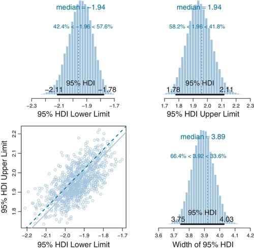
Another useful measure of the effective accuracy of the chain is the Monte Carlo standard error (MCSE). First, some background concepts and terminology. Consider randomly sampling values X₁,…,x_N from a normal distribution, and computing the mean of the sample, $\overline{x}=\frac{1}{N}{\displaystyle {\sum }_{i=1}^N{x}_i}$. The sample mean will be a noisy indicator of the underlying mean μ of the normal generating distribution. If we sample N values many times, sometimes the sample mean $\overline{x}$ will be greater than μ and sometimes less than μ. The SD of the sample mean, across repetitions, is called the standard error of the sample mean, and its estimated value is simply $\text{SE=SD}/\sqrt{N}$, where SD is the standard deviation of the sample. Thus, as the sample size increases, the standard error decreases. In other words, the bigger the sample, the less noise there is in the estimate of the underlying mean, and the standard error itselfprovides a quantitative suggestion of how big the estimation noise is. The notion of standard error for independent values is extended to Markov chains merely by substituting the ESS for the actual sample size. Thus, a simple formulation of the MCSE is

$\text{MCSE=}\text{SD}/\sqrt{\text{ESS}}$

where SD is the standard deviation of the chain and ESS is as defined in Equation 7.11. This is a simple version of MCSE; for more elaborate considerations see Flegal, Haran, and Jones (2008).

Examples of the MCSE are displayed in the lower-right panels of Figures 7.10 and 7.11. The MCSE indicates the estimated SD of the sample mean in the chain, on the scale of the parameter value. In Figure 7.11, for example, despite the small ESS, the mean of the posterior appears to be estimated very stably.

Here is a recapitulation regarding accuracy and stability of MCMC results. Visual inspection of the trace plots and density plots, and the Gelman-Rubin statistic, can suggest whether the burn-in period has been suitably passed. Second, those indicators can also suggest whether or not the chains are well mixed and representative of the posterior. Remember, the diagnostics logically can only probabilistically indicate violations of representativeness and cannot guarantee representativeness. Next, the measures of ESS and MCSE suggest how stable and accurate the chain is. As a heuristic, if you want reasonable stability in the estimates of the limits of the 95% HDI, an ESS of (at least) 10,000 is desirable. If you want a particular accuracy in the estimate of the posterior mean, consult the MCSE, which is interpreted on the scale of the parameter.

7.5.3 MCMC efficiency

The third of our main goals for MCMC is efficiency, so we do not exceed our patience and computing power. It is often the case in realistic applications that there is strong autocorrelation for some parameters, and therefore, an extremely long chain is required to achieve an adequate ESS or MCSE. There are various ways to (attempt to) improve the efficiency of the MCMC process.

• $R$un chains on parallel hardware. Most new computers have four or more processors, and each can be recruited to run a chain simultaneously, in parallel. Running parallel chains does not improve the amount of information per step in each chain, but it does improve the amount of information per increment of real time. The package runjags is nice for running parallel chains, as we will see in Chapter 8.

• Adjust the sampling method; for example, use a Gibbs sampler instead of a Metropolis sampler, as illustrated in the improvement in ESS from Figures 7.6 to 7.8. This approach requires great knowledge of various samplers and what types of model structures and substructures work best with which samplers. We will not explore these nuances in this book and will instead let sophisticated software tackle this issue for us. One sampling method that can be relatively efficient is Hamiltonian Monte Carlo, which is implemented in the Stan software introduced in Chapter 14.

• Change the parameterization of the model. In some cases, the various parameters of the model can be algebraically re-expressed in equivalent different forms but MCMC operates more efficiently in one form than another. For example, two parameters α and β might be re-expressed as μ = (α + β)/2 and δ = (α + β)/2, hence α = μ + δ and β = μ − δ. (This particular reparameterization might have little effect on MCMC sampling but is mentioned to illustrate the idea.) One application of this idea is mean-centering of data in regression analysis, as we will see in Chapter 17. We will see few other examples of this approach because applications can require a nuanced understanding of technicalities specific to individual models, which goes beyond the intended purpose of this book.

A method for reducing autocorrelation that does not improve efficiency is thinning the chain. In thinning, only every kth step in the chain is stored in the computer's memory. For example, when thinning to every 10th step, only steps 1, 11, 21, 31, and so on, are retained. The resulting thinned chain is less autocorrelated than the original complete chain. But the thinned chain also has less information than the original chain, and estimates from a thinned chain are (on average) less stable and accurate than from the original chain (Link & Eaton, 2012). After all, each step in the original chain did provide some new information. And, of course, the thinned chain takes just as many steps as the original chain to generate, so there is no savings in time during the generation of the chain. The only reason to thin a chain is if storing the full original chain would take too much computer memory, or if subsequent processing of the full original chain would take too much time.