
Chapter 5
Pattern Recognition-Based Approach for Dynamic Vulnerability Status Prediction
Jaime C. Cepeda1, José Luis Rueda-Torres2, Delia G. Colomé3 and István Erlich4
1Head of Research and Development, and University Professor, Technical Development Department, and Electrical Energy Department, Operador Nacional de Electricidad CENACE, Escuela Politécnica Nacional EPN, Quito, Ecuador
2Assistant professor of Intelligent Electrical Power Systems, Department of Electrical Sustainable Energy, Delft University of Technology, The Netherlands
3Professor of Electrical Power Systems and Control, Institute of Electrical Energy, Universidad Nacional de San Juan, Argentina
4Chair Professor of Department of Electrical Engineering and Information Technologies, Head of the Institute of Electrical Power Systems, University Duisburg-Essen, Duisburg, Germany
5.1 Introduction
Electric power systems have lately been operated dangerously close to their physical limits because of lack of investment, the use of congested transmission branches, and other technical reasons. Under these conditions, certain sudden perturbations can cause cascading events that may lead the system to blackouts. It is necessary to ensure that these perturbations do not affect security, so the requirement emerges of developing wide area protection schemes that allow guaranteeing service continuity. However, most actual wide area protection schemes are usually set to operate when specific pre-established operational conditions are reached, so they are unable to work under unconsidered contingencies that could entail cascading events. In these situations, the control of the system and the protection triggering should be adjusted depending on real-time event progress. This requirement emphasizes the need for advanced schemes to perform real-time adaptive control actions, with the aim of continuously guaranteeing system security while reducing the risk of power system blackouts [1]. Such a scheme depends upon timely and reliable provision of critical information in real time (via adequate measurement equipment and sophisticated communication networks) to quickly ascertain the system vulnerability condition (through appropriate tools to quickly analyze huge volumes of data) that subsequently allows the performance of remedial countermeasures (i.e., a Self-Healing Grid) [2]. A fundamental task of this smart structure is the real-time vulnerability assessment (VA), since this has the function of detecting the necessity of performing global control actions. Traditionally, VA approaches have been carried out to lead the system to a more secure steady-state operating condition by performing preventive control. However, in recent years, emerging technologies, such as Phasor Measurement Units (PMUs) and Wide Area Monitoring, Protection and Control Systems (WAMPAC), have enabled developing modern VA methods that permit the execution of corrective control actions [3–5]. This new framework is possible due to the great potential of PMUs to allow post-contingency dynamic vulnerability assessment (DVA) to be performed [3]. In view of this, a few PMU-based methods have been recently proposed in order to estimate the post-contingency vulnerability status by classifying real-time signal processing results obtained via application of different signal processing tools, including data mining techniques, as was presented in Chapter 1.
As highlighted in Chapter 1, the proposals discussed have not achieved good accuracy requirements due to their considerable overlap zone between stable and unstable cases. Thus, more appropriate mathematical tools should be developed in order to better adapt to power system dynamic variables and so increase the accuracy of results. In view of this, a novel approach to estimate post-contingency dynamic vulnerability regions (DVRs), taking into account three short-term stability phenomena (i.e., transient, voltage, and frequency stability—TVFS) is firstly deployed in this chapter. This proposal applies Monte Carlo (MC) simulation to recreate a wide variety of possible post-contingency dynamic data of some electrical variables, which could be available directly from PMUs in a real system (e.g., voltage phasors or frequencies). From this information, a pattern recognition method, based on empirical orthogonal functions (EOF), is used to approximately pinpoint the DVR spatial locations. Afterward, a comprehensive approach for predicting the power system's post-contingency dynamic vulnerability status is presented. This TVFS vulnerability status prediction considers the MC-based DVRs together with a support vector classifier (SVC), whose optimal parameters are determined through an optimization problem solved by the swarm version of the mean-variance mapping optimization (MVMOS).
5.2 Post-contingency Dynamic Vulnerability Regions
As stated in Chapter 1, most existing VA methods are based on steady-state (Static Security Assessment—SSA) or dynamic (Dynamic Security Assessment—DSA) simulations of N-x critical contingencies. The aim of these methods is to determine whether the post-contingency states are within a “safe region” [4, 6] and accordingly to decide the most effective preventive control actions.
For this purpose, a Dynamic Security Region (DSR) might be established in order to determine the feasible operating region of an Electric Power System [6]. The process consists in determining the boundary of the DSR, which can be approximated by hyper-planes [6], and specifying the actual operating state relative position (or “security margin”) with respect to the security boundary [4].
A fast direct method is presented in [6] in order to compute the DSR hyper-plane boundary for transient stability assessment (TSA) and to enhance the system stability margin by performing appropriate preventive strategies. Also, an approach to achieve on-line VA by tracking the boundary of the security region is outlined in [7]. These approaches have been focused on analyzing only one electrical phenomenon (commonly TSA), with the goal of leading the system to a more secure steady-state operating condition (by performing preventive control).
The concept of DSR has been used in order to define a method for security assessment. In this sense, DSA is defined as “the determination of whether the actual operating state is within the DSR.” The DSR can be defined in the injection space, depending on the analysis of TSA [6]. This DSR can be approximated by hyper-planes, and the computation of their boundaries allows specifying the “security margin” with respect to them [6]. The aim of this assessment is to enhance the system stability margin through performing appropriate preventive control actions.
Using the same concept as DSR, a DVR is defined in this chapter in order to perform post-contingency DVA with the aim of conducting corrective control actions. This DVR can also be specified by hyper-planes as in (5.1):
where x is an n-dimensional vector, and c is a constant that represents the value of the DVR boundary [7].
Figure 5.1 illustrates the DVR concept, where the DVR boundary delimits the “vulnerable” and the “non-vulnerable” regions.
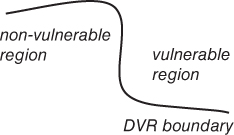
Figure 5.1 Dynamic vulnerability region concept.
The DVR and the hyper-plane boundaries of a dynamic system can be determined analytically or numerically. However, due to the huge complexity of bulk power systems, determining their DVRs analytically is not possible [7]. In this case, numerical methods offer the possibility of considering the complex power system physical model through simulation of several dynamic operating states. Monte Carlo methods are appropriate for analyzing the complexities in large-scale power systems with high accuracy, at the expense of greater computational effort [8].
By applying the introduced DVR concept, this chapter describes a novel approach to determining the post-contingency TVFS vulnerability status of an Electric Power System. This proposal allows assessing the second task related to real-time post-contingency DVA, which is the prediction of the system's tendency to change its conditions to a critical state.
5.3 Recognition of Post-contingency DVRs
With the aim of numerically determining the power system DVR and its hyper-plane boundaries, Monte Carlo-type (MC) simulation is performed to iteratively evaluate the post-contingency system time domain responses. In order to perform MC-based simulations, several input data are required. These data depend on the objective of the simulation, and they are usually represented by their corresponding probability distribution functions (PDFs). Since the proposal constitutes a wide area real-time post-contingency situational awareness methodology, capable of being updated even daily by the independent system operator (ISO) in the control center, the proposed uncertainty analysis encompasses only a specific short-term planning horizon. Thus, the probabilistic models of power system random variables, as well as the grid topology, should be structured within this short-term planning horizon so as to reflect the behavior of the system as realistically as possible.
In this connection, the basic data to be considered in the MC-based simulation, and which have to be previously prepared by the system operator, are: (i) short-term forecasting of nodal loads, (ii) short-term unit commitment, (iii) short-term system topology, and (iv) random generation of N-1 contingencies. Based on these system operating definitions, MC-type simulation is performed to iteratively evaluate the system responses, which would resemble those signals recorded in real time by smart metering, for instance by PMUs located throughout the system, with the ultimate goal of structuring a performance database.
Therefore, MC-based simulation is proposed as a method to obtain post-contingency data of some electrical variables, which would be available directly from PMUs in a real system (i.e., voltage phasors or frequencies), considering several possible operating conditions and contingencies including the most severe events that could lead the system to potential insecure conditions, and subsequent cascading events. Therefore, dynamic N-1 contingency simulations are performed via the MC-process, as depicted in Figure 5.2. First, the input variables to be considered in the MC simulation are randomly generated from the appropriate PDFs: that is, the load in each bus, the type of contingency (e.g., short circuit, generation outage, or load event), the faulted element (line, generator, or load), and the short circuit location, or the amount of load to be changed, or the branch outage in the case of static contingency analysis. Then, optimal power flow (OPF) is performed for every trial set of input variables in order to define feasible pre-contingency steady-state scenarios. Afterward, N-1 dynamic contingency time domain simulations are performed in order to obtain the post-contingency dynamic data that have led to the post-contingency dynamic vulnerability system status. These dynamic probabilistic attributes are then analyzed using a time series data mining technique based on EOFs, in order to recognize the system DVRs based on the patterns associated to the three short-term TVFS phenomena. This procedure is schematically summarized in Figure 5.2.

Figure 5.2 Methodological framework for recognition of DVRs.
The ultimate goal of the methodology presented in Figure 5.2 is to map the spatial distribution of the DVRs, as well as to determine the EOFs that constitute the best orthogonal functions for extracting the predominant patterns buried in the post-contingency signals. These EOFs will be then used in real time in order to transform the actual measured signal into its corresponding pattern vector (by means of the projection of the data in the direction of the main EOFs), which has led to the information of the system post-contingency vulnerability status.
5.3.1 N-1 Contingency Monte Carlo Simulation
The DVRs are proposed in order to take advantage of the great potential of PMUs to allow performing post-contingency DVA that can be used to trigger corrective control actions in real time. Conventionally, these corrective actions are set to occur when specific pre-established operational conditions are reached, and they are unable to work under unconsidered contingencies that could begin cascading events.
Monte Carlo simulation allows obtaining the dynamic PMU post-contingency variables, which are used to determine the DVRs for the bulk power system under analysis. Figure 5.2 depicts the Monte Carlo simulation procedure in detail.
In order to adequately apply Monte Carlo simulation and obtain realistic results of the post-contingency dynamic response, some considerations and modeling requirements are taken into account:
- The DVRs can be defined for either short-term or long-term phenomena. This chapter focus on the three phenomena defined as short-term stability, which comprises transient stability, short-term voltage stability, and short-term frequency stability (TVFS) [9].
- Since the accuracy of the DVR boundaries depends on the accuracy of the models, the dynamic components (generators, motors, loads) and relevant control systems (such as excitation control system and speed governor systems) must be modeled with enough detail [8].
- The simulated events are based on N-1 contingencies, and the vulnerability criterion consists in the possibility of this kind of disturbance driving the system to further undesirable events (i.e., N-2 contingencies), which are considered as the beginning of a cascading event. For this purpose, three types of local protection devices are modeled in this chapter: out-of-step relays (OSR), under and over voltage relays (VR), and under and over frequency relays (FR). The tripping of one or more of these protection relays is used as the indicator of an imminent cascading event, and so it becomes a sensor of system vulnerability status. Thus, after each MC iteration, a vulnerability status flag gets the value of “1” (i.e., status of vulnerable) if one or more of the above mentioned local protections were tripped during the time domain simulation. Otherwise, in the case that none of the local protections was tripped, this vulnerability status flag acquires the value of “0” (i.e., status of non-vulnerable). This vulnerability status indicator is stored together with the post-contingency dynamic data. At the end of the MC simulation, a vulnerability status vector (vs) will contain all the vulnerability status flags corresponding to each iteration.
5.3.2 Post-contingency Pattern Recognition Method
The required mathematical tool for achieving the tasks involved in the post-contingency DVA has to be capable of predicting the post-contingency system security status and of specifying the actual dynamic state relative position with respect to the DVR boundaries, with reduced computational effort and quick-time response. Pattern recognition-based methods have the potential to effectively achieve this goal.
Pattern recognition is concerned with the automatic discovery of similar characteristics in data by applying computer algorithms and using them to take some action such as classifying the data into different categories [10], called classes [11].
Dynamic electrical signals can exhibit certain regularities (patterns) signalling a possibly vulnerable condition. However, these patterns are not necessarily directly evident in the electrical signal, though it may contain hidden information which can be uncovered by a proper pattern recognition tool [3].
This chapter applies a novel methodology for recognizing patterns in post-contingency bus features in order to numerically determine the DVRs of a specific Electric Power System. The method uses a time series data mining technique based on EOFs. The data consist of measurements of some dynamic post-disturbance PMU variables (voltage phasors or frequencies) at m spatial locations (buses where PMUs are installed) at r different times of n Monte Carlo cases. The measurements are arranged so that p time measures are treated as variables (![]() ) and every Monte Carlo simulation plays the role of observation, constituting an (
) and every Monte Carlo simulation plays the role of observation, constituting an (![]() ) time series data matrix (F).
) time series data matrix (F).
In the case of voltage angles, and since transient stability depends on angle separation, it is recommended not to use the voltage angles directly but to employ normalized angles obtained via the previous application of (5.2):
where xi(t) represents the voltage angle on bus i at time t; xi0 is its initial value prior to the perturbation; and ![]() is the average value over the number of buses Nb at time t:
is the average value over the number of buses Nb at time t:

Once matrix F has been structured, the method for obtaining EOFs is applied to this matrix. EOFs are the result of applying singular value decomposition (SVD) to time series data [12, 13]. Some authors consider that Principal Component Analysis (PCA) and EOF are synonymous [13]; nevertheless, this chapter uses a different interpretation of these two techniques. Whereas PCA is a data mining method that allows reducing the dimensionality of the data, EOF is a time series data mining technique that allows decomposing a discrete function of time f(t) (such as voltage angle, voltage magnitude, or frequency) into a sum of a set of discrete pattern functions, namely EOFs. Thus, EOF transformation is used in order to extract the most predominant individual components of a compound signal waveform (similar to Fourier analysis), which allows revealing the main patterns buried in the signal.
The main approaches related to EOFs have been developed for use in the analysis of spatio-temporal atmospheric science data, whereas their application in other scientific fields continues to be scarce. The data concerned consist of measurements of specific variables (such as sea level pressure, temperature, etc.) at n spatial locations at p different times [14]. As mentioned before, this chapter employs a variation of this definition, where the n spatial locations are replaced by n different post-contingency power system states (obtained from MC simulation), and the p different times consist of PMU instant values of post-disturbance dynamic variables (voltage phasors or frequencies) measured on m buses, at r different instants that depend on the selected time window (i.e., ![]() ).
).
Therefore, an (![]() ) data matrix of discrete functions (F) is structured, where the post-contingency measurements at different power system states (n) are treated as observations, and the PMU samples belonging to a pre-specified time window (p time points) play the role of variables. Since the different power system states result from the application of MC-based simulations, n is conceptually greater than
) data matrix of discrete functions (F) is structured, where the post-contingency measurements at different power system states (n) are treated as observations, and the PMU samples belonging to a pre-specified time window (p time points) play the role of variables. Since the different power system states result from the application of MC-based simulations, n is conceptually greater than ![]() , and so F is a rectangular matrix:
, and so F is a rectangular matrix:

where fk is the k-th discrete function of time obtained in the k-th MC-repetition that consists of p samples.
Formally, the SVD of the real rectangular matrix F of dimensions (![]() ) is a factorization of the form [15]
) is a factorization of the form [15]
where U is an orthogonal matrix whose columns are the orthonormal eigenvectors of FF′, V′ is the transpose of an orthogonal matrix whose columns are the orthonormal eigenvectors of F′F, and Λ1/2 is a diagonal matrix containing the square roots of eigenvalues from U or V in descending order, which are known as the singular values of F.
Taking into account that ![]() , this matrix decomposition can be written, as a finite summation, as follows:
, this matrix decomposition can be written, as a finite summation, as follows:

where ui and vi are the i-th column eigenvectors belonging to U and V respectively, and λi1/2 is the i-th singular value of F.
From (5.6), and after some computations, each element of F (each discrete function) can be written as follows:
It is worth mentioning that the expression shown by (5.7) actually represents the decomposition of the discrete function of time fk into a sum of a set of discrete functions (vj) which are orthogonal in nature (since they are the orthonormal eigenvectors of F′F), weighted by real coefficients resulting from the product of the j-th singular value of F by the j-th element of the eigenvector uk. Thus, vj represents the j-th EOF and its coefficient ![]() is called the EOF score.
is called the EOF score.
Based on a generalization of (5.7), it is possible to reconstruct the complete matrix F (i.e., the original data) using the EOFs and their corresponding EOF scores as given in (5.8):

where ai is the i-th vector whose elements are all the aij EOF scores.
Comparing (5.6) and (5.8), it is easily concluded that ![]() . Then, all aij EOF scores can be calculated by using its matrix form as follows:
. Then, all aij EOF scores can be calculated by using its matrix form as follows:
where A is the EOF score matrix.
From (5.5) and (5.9), it can be determined that
From the last equation, and based on the fact that V is an orthogonal matrix (whose main feature is that its transpose is equal to its inverse), the EOF score matrix A can be computed by (5.11):
where matrix V contains the corresponding EOFs of F (i.e., the eigenvectors of F′F).
The sum of the singular values of F (λi1/2) is equivalent to the total variance of the data matrix, and each i-th singular value offers a measurement of the explained variability (EVi) given by EOFi as defined by (5.12). Thus, the number of the chosen EOFs depends on the desired explained variability:

It is worth mentioning that the main advantage of EOFs is their ability to determine the orthogonal functions that better adapt to the set of dynamic functions. This feature enables the mining of the patterns in the signal, and allows EOF to beat other signal processing tools such as Fourier analysis, which always employs the same pre-defined trigonometric pattern functions (i.e., sine and cosine), which are not always suited to representing specific dynamic behavior [16].
Once the EOFs (coefficients and scores) are computed, the corresponding EOF scores represent the projection of the data in the direction of the EOFs and form vectors of real numbers that represent the post-contingency dynamic behavior of the system. These pattern vectors permit mapping of the DVRs represented in the coordinate system formed by the EOFs.
Additionally, since some features in greater numeric ranges can dominate those of smaller numeric ranges, a numerical normalization is recommended before mapping the DVRs. Then, the pattern vectors have to be scaled in order to avoid this drawback [17]. In this chapter, a linear scaling in the range of [0, 1] is proposed.
Each pattern vector has a specific associated “class label” depending on the resulting vulnerability status vector (vs). These class labels might correspond to a non-vulnerable case (label 0) or a vulnerable case (label 1). Using the resulting pattern vectors and their associated vulnerability status class labels, the DVRs can be numerically mapped in the coordinate system formed by the main EOFs. Figure 5.3 presents the scheme of the proposed post-contingency pattern recognition method.

Figure 5.3 Post-contingency pattern recognition method.
5.3.3 Definition of Data-Time Windows
In order to adequately show the system response for the different stability phenomena, several time windows (TWs) have to be defined. These time windows are established depending on the Monte Carlo statistics of the relay tripping times, influenced also by the WAMPAC communication time delay (tdelay), which represent the delays caused by measurement, communication, processing, and tripping. It is noteworthy that TW corresponds to the length of each time window, whose beginning (t0) always accords with the instant of the fault clearing (tcl).
Since three different types of relays are considered, three different tripping time statistical analyses will be carried out. First, the minimum MC tripping time (tmin) has to be determined. This time represents the maximum admissible delay for the actuation of any corrective control action, which has to be also affected by the WAMPAC communication time delay:
where tOSRi, tVRi, and tFRi are the tripping times of OSRs, VRs, and FRs of the n MC repetitions, respectively. Typically, OSRs present the fastest tripping time due to the fast time-frame evolution of TS.
Since the post-contingency data comprise the samples taken immediately after the fault is cleared, the first time window (TW1) is defined by the difference between tmin and the clearing time (tcl):
The rest of the time windows are defined based on the statistical concept of confidence interval related to Chebyshev's inequality [18], which requires that at least 89% of the data lie within three standard deviations (3σ):
where std{·} represents the standard deviation (σ) of the relay tripping time that most intersects the corresponding time window TWk.
5.3.4 Identification of Post-contingency DVRs—Case Study
For illustrative purposes, this section shows the recognition of the post-contingency DVRs of the IEEE New England 39-bus, 60 Hz [19] and 345 kV test system, slightly modified in order to satisfy the N-1 security criterion and to include dynamic load models, automatic voltage regulators (AVR), governors (GOV), and the three mentioned types of relays: OSR, VR, and FR. Additionally, six PMUs have already been located at buses 2, 9, 11, 17, 22, and 28, based on the results presented in [20]. The test system single-line diagram is depicted in Figure 5.4, which also includes the PMU location.
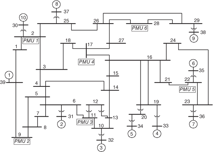
Figure 5.4 IEEE New England 39-Bus test system single-line diagram [19].
The placement PMUs are considered to have a one-cycle (16.67 ms) updating period. Also, it is assumed that the WAMPAC communication time delay is ![]() (i.e., a conservative value derived from the reference data presented in Chapter 1).
(i.e., a conservative value derived from the reference data presented in Chapter 1).
Simulations were carried out in DIgSILENT PowerFactory and consisted of several contingencies where the causes of vulnerability could be transient instability, short-term voltage instability, or short-term frequency instability (TVFS). These contingencies are generated by applying the Monte Carlo method.
Two types of events are considered: three phase short circuits and generator outage. The short circuits are applied at different locations of the transmission lines, depending on the Monte Carlo simulation. The disturbances are applied at 0.12 s, followed by the opening of the corresponding transmission line at 0.2 s (i.e., 80 ms fault clearing time tcl). Likewise, the generator to be tripped is also chosen by the Monte Carlo method, and this type of contingency is applied at 0.2 s. Several operating states have been considered by varying the loads of PQ buses, depending on three different daily load curves. Then, optimal power flow (OPF) is performed in order to establish each operating state, using the MATPOWER package. After that, time domain simulations have been performed using the DIgSILENT PowerFactory software, so that the post-contingency PMU dynamic data could be obtained.
Both voltage components (magnitude and angle), and bus frequencies are considered as potential input variables. A total number of 10 000 cases have been simulated, from which 7600 are stable or “non-vulnerable” and 2400 are unstable or “vulnerable”: 1308 are transient unstable, 682 are frequency unstable, and 410 are voltage unstable. It is worth to mention that 84 cases belonging to the 7600 TVFS non-vulnerable instances correspond to oscillatory unstable cases. Nevertheless, since oscillatory phenomena are treated in a different way in this book, these affairs will be separately analyzed in Chapter 6.
For illustrative purposes, the post-contingency dynamic responses of two different MC iterations are presented in Figures 5.5 and 5.6. These figures depict the simulation results of one non-vulnerable case and one voltage unstable case (vulnerable case). It is possible to observe in the figures the particular signal dynamic behavior for each case, which expose the existence of certain patterns revealing the actual system security level as well as the future system vulnerability status tendency.

Figure 5.5 39-bus-system: non-vulnerable case

Figure 5.6 39-bus-system: voltage unstable case.
By using the MC simulation results, consisting of the post-contingency PMU dynamic data, the relay tripping times, and the vulnerability status vector, the DVRs are identified for this specific power system. First, several time windows are defined based on the Monte Carlo statistics of the relay tripping times. Figure 5.7 presents the 39-bus-system relay tripping time histograms, where the reference frame corresponds to the time simulation.

Figure 5.7 Relay tripping time Histograms for 39-bus-system: (a) OSR, (b) VR, (c) FR.
The out-of-step relay time has a mean of 1.2252 s, a standard deviation of 0.3746 s, and a minimum value of 0.8342 s. Thus, vulnerability assessment has to be done in less than 0.5842 s (![]() ). For this reason, an adequate data window (TW1) for TS phenomenon would be 300 ms (
). For this reason, an adequate data window (TW1) for TS phenomenon would be 300 ms (![]() ) starting from fault clearing.
) starting from fault clearing.
In this test system, the tripping of voltage relays presents a mean of 4.1275 s, a standard deviation of 1.6872 s, and a minimum value of 3.22 s, whereas the frequency relay tripping time has a mean of 10.6829 s, a standard deviation of 2.4921 s, and a minimum value of 5.987 s. Using these values, and (5.15), the rest of the time windows are determined. This time window definition is summarized in Table 5.1.
Table 5.1 Time window definition for 39-bus-system
| TimeWindow | std{tOSR/VR/FR} (s) | TW(s) | |
| TW1 | – | – | 0.30 |
| TW2 | 0.3746 | 1.4238 | 1.50 |
| TW3 | 0.3746 | 2.6238 | 2.70 |
| TW4 | 0.3746 | 3.8238 | 3.90 |
| TW5 | 1.6872 | 8.9616 | 9.00 |
After TW definition, the corresponding EOF coefficients and scores (i.e., pattern vectors) are determined using the resulting MC dynamic data. After this, the EOF scores are computed. For instance, the first four TW3 voltage-magnitude-based EOFs are presented in Figure 5.8. Similarly, EOFs are determined for each electric variable at every TW.

Figure 5.8 TW3 voltage-magnitude-based EOFs for 39-bus-system: (a) EOF 1, (b) EOF 2, (c) EOF 3, (d) EOF 4.
Once the EOF scores are computed, the corresponding DVRs can be mapped. For instance, Figure 5.9 presents the three dimensional distribution of the pattern vectors obtained from the voltage magnitudes corresponding to TW3. In the figure, the ellipsoidal area (enclosing the “vulnerable” pattern vectors represented by circles) represents the vulnerable region; whereas the white area (relating to the “non-vulnerable” diamond pattern vectors) corresponds to the non-vulnerable region.

Figure 5.9 TW3 voltage-magnitude-based DVRs for 39-bus-system.
These areas have been empirically delimited, bordering the obtained pattern shapes which depend on the pattern vector spatial locations. The plot presents the DVRs corresponding to the first three EOFs depicted in Figure 5.8.
5.4 Real-Time Vulnerability Status Prediction
The DVRs will be used to specify the actual dynamic state relative position with respect to their boundaries, which might be established using an intelligent classifier. For this purpose, a support vector classifier (SVC) is proposed in this chapter since this classifier computes an optimal hyper-plane that separates the vector space depending on the spatial location of each class [11, 21]; this agrees with the hyper-plane-based definition of DVRs laid out in Section 5.2. Additionally, the SVC has the property of being more robust in avoiding over-fitting problems [8], which is also desirable in order to get enough robustness and generalization in classifying an actual case in real time. This classifier acquires decision functions that classify an input into one of the given classes through training using input-output (features-label) pair data. The optimal decision function is called the Optimal Hyper-plane (OH), and it is determined by a small subset of the training set which are called the Support Vectors (SV), using the concept of the VC (Vapnik–Chervonenskis) dimension as the theoretical basis [11]. Figure 5.10 shows an illustration of an SVC solution for a two-class data classification problem, where the SV and the OH have been determined. The classified vectors belong to one of two different groups, that is, “class 1” or “class 2,” and they are represented in a two-dimensional plane whose axes are the first and second variables (x1 and x2) of the feature vectors (x).

Figure 5.10 Support vectors and optimal separating hyper-plane of SVC.
The SVC needs an a priori off-line learning stage, in which the classifier has to be trained using a training set of data. Hence, the data have to be split into training and testing sets. Each element in the training set contains one “target value” (class labels) and several “attributes” (features). The objective of the SVC is to yield a training data based model, which predicts the target values of the test data given only the test data features [17].
Given a training set of features-label pairs ![]() where
where ![]() and
and ![]() , for a two-class classification problem, the support vector classifier requires the solution of the optimization problem shown in (5.16) [17]:
, for a two-class classification problem, the support vector classifier requires the solution of the optimization problem shown in (5.16) [17]:

where w is an n-dimensional weight vector, b is a bias term, ξi is a slack variable associated with xi, C is the margin parameter, and φ(xi) is the mapping function from x to the feature space [11]. It is worth mentioning that w, b, and ξi are determined via the SVC optimization process, whereas C is a parameter to be specified a priori.
The mapping function φ(xi) is usually defined as the so called “kernel function” K(xi, xj), as in (5.17) [17]:
There are several types of kernel function, such as linear, polynomial, and radial basis function (RBF), among others. Figure 5.10 presents, for instance, an OH determined using a linear kernel function.
In this chapter, an RBF kernel (5.18) is used because it is capable of handling possible nonlinear relations between labels and features [17]:
Before training the SVC, it is necessary to identify the best parameters C of (5.16), and γ of (5.18) [17], as well as Wm that represents a weight factor used to change the penalty of class m, which is useful for training classifiers using unbalanced input data [21]. For this purpose, an optimization problem is solved via the swarm version of the mean-variance mapping optimization (MVMOS), for which the details of implementation can be obtained from [22].
Based on the requirement of dynamic vulnerability status prediction, a two-class classifier is structured that sorts the power system vulnerability status into “vulnerable” or “non-vulnerable” using the pattern vectors obtained from the pattern recognition method as inputs of SVC. The classifier needs an a priori off-line learning stage, in which SVC has to be trained using the previously recognized DVRs (i.e., pattern vectors and vulnerability status). For real-time implementation, the classifier uses the post-contingency voltage phasors (angles and magnitudes) and frequencies, obtained from the PMUs, transformed by the EOFs stored in the control center processor as table-based reference functions. Then, the classifier will classify the system's tendency to become “vulnerable” or “non-vulnerable.”
Figure 5.11 presents a flowchart of the proposed real-time vulnerability status classification algorithm, including the off-line training stage.

Figure 5.11 Post-contingency vulnerability status prediction methodology.
5.4.1 Support Vector Classifier (SVC) Training
In dynamic vulnerability status classification, the target values resemble the MC vulnerability status “class label.” These class labels might correspond to non-vulnerable cases (label 0) or vulnerable cases (label 1), depending on the triggering status of the different relays. Hence, a two-class classifier has to be used. The attributes, instead, are represented by the post-contingency pattern vectors that better represent the DVRs belonging to each time window. In this connection, and based on the fact that some signals better show the evolution of specific phenomena than others, a procedure for improving the feature extraction and selection has to be followed in order to choose the appropriate pattern vectors before training the SVC. Then, it is necessary to choose an adequate number of EOFs that allows maintaining as much of the variation presented in the original variables as possible. This analysis constitutes the proposed feature extraction stage. For this purpose, the i-th EOF desired explained variability (EVi), represented by (5.12), is used as a weight measure. After several tests, it has been established that the number of EOFs chosen will be that which permits obtaining an EVi of more than 97%. In the case where the EVi requirement is satisfied already with the first EOF, two EOFs will be used in order to ensure the mapping of at least two-dimensional DVRs. On the other hand, based on the premise that some electrical variables better show the evolution of specific phenomena than others, it is necessary to select those signals that allow the best DVR representation for each TW. The selection will permit obtaining the best classification accuracy. This analysis can be seen as the feature selection stage. Therefore, a decision tree (DT) method for feature selection, originally introduced in [23], has been adapted to this problem, based on the classification accuracy obtained considering a combinatorial analysis of the potential electrical variables. Additional details of this feature extraction and feature selection method can be found in [22].
Once the optimal SCV parameters have been identified and the best features have been determined, the SVC is trained for each data-time window. The objective is to obtain a robust enough SVC that allows predicting the vulnerability status by using as input the best pattern vectors obtained from the EOFs. For this purpose, 10-fold cross validation (CV) is used to analyze the robustness of the classifier training as explained in [22]. For illustrative purposes, the performance of the trained SVC for each of the five TW determined in the previously presented case study is presented in Table 5.2. This table also includes the performance of other classifiers, such as: decision tree classifier (DTC), pattern recognition network (PRN: a type of feed-forward network), discriminant analysis (DA), and probabilistic neural networks (PNN: a type of radial basis network). The performance of the classification is evaluated, in this comparison, by means of the mean of each CV-fold classification accuracy (CAi) for each TW [22]. The Library for Support Vector Machines (LIBSVM) [21] is used for designing, training, and testing the SVC models.
Table 5.2 Classification performance of 39-bus-system
| mean{CAi} for Time Window (%) | |||||
| Classifier | TW1 | TW2 | TW3 | TW4 | TW5 |
| DA | 97.440 | 99.966 | 99.494 | 98.034 | 97.178 |
| DTC | 98.200 | 99.931 | 99.736 | 99.436 | 99.291 |
| PRN | 98.760 | 99.897 | 99.770 | 99.029 | 98.993 |
| PNN | 98.930 | 99.977 | 99.770 | 99.137 | 99.055 |
| SVC | 99.290 | 100.00 | 99.885 | 99.880 | 99.727 |
From the results, it is possible to observe that the SVC outperforms all other classifiers in terms of classification accuracy. In addition, the SVC is the only classifier that permits obtaining more than 99% of CA for all TWs. These results allow us to form the conclusion that the SVC presents an excellent performance when adequate parameters and features are used. Then, suitable parameters permit exploiting the SVC advantage of being more robust to over-fitting problems, which is reflected in a more robust 10-fold CV accuracy. This pre-requisite has been optimally satisfied via the proposed MVMOS-based parameter identification method.
5.4.2 SVC Real-Time Implementation
For real-time implementation, the off-line trained SVCs will be in charge of classifying the post-contingency dynamic vulnerability status of the power system, using the actual post-contingency PMU voltage phasors and frequencies as data. First, the dynamic signals must be transformed to the corresponding EOF scores. For this purpose, the measured data have to be multiplied by the EOFs determined in the off-line training and stored in the control center processor. Then, the obtained EOF scores will be the input data to the trained SVCs, which will automatically classify the system status into “vulnerable” or “non-vulnerable.” This vulnerability status prediction will be then used by the “performance-indicator-based real-time vulnerability assessment” module (for more details, see Chapter 6) that is responsible for computing several vulnerability indices, which are the final indicators of the system vulnerability condition. Since this classification uses patterns hidden in the input signal as input data, it is capable of predicting the post-contingency dynamic vulnerability status before the system reaches a critical state. Then, the methodology presented in this chapter allows the assessment of the second aspect regarding the vulnerability concept, whose causes concern TVFS issues. Figure 5.12 illustrates how the proposed TVFS vulnerability status prediction method might be implemented in a control center.

Figure 5.12 SVC real-time implementation in a control center.
In order to validate the complete TVFS vulnerability status prediction presented in this chapter, the power system protection concepts of dependability (Dep (5.19): ability for tripping when there exists the necessity to trip) and security (Sec (5.20): ability not to trip when there is no necessity to trip) are used. It is worth mentioning that security is more critical than dependability because a miss-classification might suggest wrong corrective control actions:


Table 5.3 shows a summary of the number of vulnerable and non-vulnerable cases corresponding to the case study of the 39-bus system, where the percentages of complete classification accuracy, security, and dependability are also presented. Results highlight the excellent performance of the methodology regarding security and dependability, offering more than 99% confidence in both measures. The small percentage of errors is due to the existence of overlapping zones between vulnerable and non-vulnerable regions.
Table 5.3 Vulnerability status prediction performance for 39-bus-system
| Feature | Value |
| Non-vulnerable cases correctly classified | 7587 |
| Vulnerable cases correctly classified | 2390 |
| Non-vulnerable cases classified as vulnerable | 13 |
| Vulnerable cases classified as non-vulnerable | 10 |
| Complete classification accuracy (%) | 99.770 |
| Security (%) | 99.829 |
| Dependability (%) | 99.583 |
Considering the necessity of ensuring very quick response for WAMPAC applications, the methodology presented in this chapter must deliver in a very short elapsed time. Thus, in order to verify the speed of the real-time computations of the proposed method, a complete classification test has been made using only one of the cases analyzed in the previous simulations, which would represent a real-time event. Simulations have been run in Windows 7 Ultimate-Intel (R) Core (TM) i3-2350M-2.30GHz-6GB RAM. In this instance, the resulted SVC elapsed time was 0.68 ms, and the entire process presented in Figure 5.12 takes only 1.47 ms. This very quick response of the proposed methodology matches the very short time delay requirement of this type of real-time application.
5.5 Concluding Remarks
This chapter presents a novel post-contingency pattern recognition method for predicting the dynamic vulnerability status of an Electric Power System. The methodology begins with the determination of post-contingency DVRs using MC simulation and EOFs, which allow finding the best pattern functions for representing the particular dynamic signal behavior. This proposal considers three different short-term instability phenomena as the potential causes of vulnerability (TVFS), for which several time windows have been defined. These DVRs are then used to specify the actual dynamic state relative position with respect to their boundaries, which is established using an intelligent classifier together with an adequate feature extraction and selection scheme. In this connection, SVC is used due to its property of being particularly robust to over-fitting problems when adequate parameters and features are selected. From the results, it is possible to observe that the post-contingency TVFS vulnerability status prediction method permits assessment of the second aspect regarding the vulnerability concept by analyzing the system's tendency to reach an unstable condition with high classification accuracy and low time-consumption requirements. In addition, this mathematical tool has been capable of predicting system response using only small windows of post-contingency data obtained directly from PMUs located in some high voltage transmission buses. Thus, it is not necessary to calculate other physical variables (e.g., rotor angles or machine rotor speeds), which are needed in the traditional TSA. The obtained classification accuracy (more than 99%) outperforms the few methods reported by the literature that also aim to estimate system vulnerability status via the application of other types of signal processing techniques (such as Short Time Fourier Transform (STFT) [24] or Local Correlation Network Pattern (LCNP) [25], as discussed in Chapter 1), in which the considerably large overlap zone provokes confusion between vulnerable and non-vulnerable regions. The presented approach, in contrast, allows a better adaptation of the system dynamic variables of interest by using empirical orthogonal functions based on the fact that this technique permits finding the best pattern functions for representing the particular signal dynamic behavior. In this manner, an improvement in the accuracy of classification results is obtained compared to the application of other signal processing tools, such as STFT or LCNP. The TVFS vulnerability status prediction presented in this chapter is not alone sufficient to achieve recognition of the specific symptom of system stress that is the cause of the vulnerability, which might help in orienting the adequate corrective control action. Hence, the need to use some complementary decision techniques (e.g., Key Performance Indicators (KPIs)) that allow an increase in security confidence and permit recognizing the causal symptoms of vulnerability; these will be discussed in Chapter 6 of this book. This complementary analysis, based on performance indices, will help toward better decision making.
References
- 1 K. Moslehi, and R. Kumar, “Smart Grid – A Reliability Perspective”, IEEE PES Conference on Innovative Smart Grid Technologies, January 19–20, 2010, Washington, DC.
- 2 M. Amin, “Toward Self-Healing Infrastructure Systems”, Electric Power Research Institute (EPRI), IEEE, 2000.
- 3 J. C. Cepeda, D. G. Colomé, and N. J. Castrillón, “Dynamic Vulnerability Assessment due to Transient Instability based on Data Mining Analysis for Smart Grid Applications”, IEEE PES ISGT-LA Conference, Medellín, Colombia, October 2011.
- 4 S. C. Savulescu, et al, Real-Time Stability Assessment in Modern Power System Control Centers, IEEE Press Series on Power Engineering, Mohamed E. El-Hawary, Series Editor, a John Wiley & Sons, Inc., Publication, 2009.
- 5 Z. Huang, P. Zhang, et al, “Vulnerability Assessment for Cascading Failures in Electric Power Systems”, Task Force on Understanding, Prediction, Mitigation and Restoration of Cascading Failures, IEEE PES Computer and Analytical Methods Subcommittee, IEEE Power and Energy Society Power Systems Conference and Exposition 2009, Seattle, WA.
- 6 Y. Zeng, P. Zhang, M. Wang, H. Jia, Y. Yu, and S. T. Lee, “Development of a New Tool for Dynamic Security Assessment Using Dynamic Security Region”, 2006 International Conference on Power System Technology.
- 7 M. A. El-Sharkawi, “Vulnerability Assessment and Control of Power System”, Transmission and Distribution Conference and Exhibition 2002: Asia Pacific., Seattle, WA, USA, Vol. 1, pp. 656–660, October 2002.
- 8 Z. Dong, and P. Zhang, Emerging Techniques in Power System Analysis, Springer, 2010.
- 9 P. Kundur, J. Paserba, V. Ajjarapu, et al, “Definition and Classification of Power System Stability”, IEEE/CIGRE Joint Task Force on Stability: Terms and Definitions. IEEE Transactions on Power Systems, Vol. 19, pp. 1387–1401, August 2004.
- 10 C. Bishop, Pattern Recognition and Machine Learning, Springer, 2006.
- 11 S. Abe, Support Vector Machines for Pattern Classification, Second Edition, Springer, 2010.
- 12 E. N. Lorenz, “Empirical Orthogonal Functions and Statistical Weather Prediction”, Statistical Forecasting Project Rep. 1, MIT Department of Meteorology, 49 pp, December 1956.
- 13 H. Björnsson, and S. Venegas, “A Manual for EOF and SVD Analyses of Climatic Data”, C2GCR Report No. 97-1, McGill University, February 1997, [Online]. Available at: http://www.geog.mcgill.ca/ gec3/wp-content/uploads/2009/03/Report-no.-1997-1.pdf.
- 14 I. Jollife, Principal Component Analysis, 2nd. Edition, Springer, 2002.
- 15 D. Peña, Análisis de Datos Multivariantes, Editorial McGraw-Hill, España.
- 16 J. Cepeda, and G. Colomé, “Benefits of Empirical Orthogonal Functions in Pattern Recognition applied to Vulnerability Assessment”, IEEE Transmission and Distribution Latin America (T&D-LA) 2014, Medellín, Colombia, Septiembre 2014.
- 17 C-W. Hsu, C-C. Chang, and C-J. Lin, “A Practical Guide to Support Vector Classification”, April 15, 2010, [Online]. Available: http://www.csie.ntu.edu.tw/∼cjlin.
- 18 J. Han, and M. Kamber, Data Mining: Concepts and Techniques, second edition, Elsevier, Morgan Kaufmann Publishers, 2006.
- 19 M. A. Pai, Energy Function Analysis for Power System Stability, Kluwer Academic Publishers, 1989.
- 20 J. Cepeda, J. Rueda, I. Erlich, and G. Colomé, “Probabilistic Approach-based PMU placement for Real-time Power System Vulnerability Assessment”, 2012 IEEE PES Conference on Innovative Smart Grid Technologies Europe (ISGT-EU), Berlin, Germany, October 2012.
- 21 C-C. Chang, and C-J. Lin, “LIBSVM: A Library for Support Vector Machines”, 2001. [Online]. Software Available at: http://www.csie.ntu.edu.tw/∼cjlin/libsvm.
- 22 J. Cepeda, J. Rueda, G. Colomé, and I. Erlich, “Data-Mining-Based Approach for Predicting the Power System Post-contingency Dynamic Vulnerability Status”, International Transactions on Electrical Energy Systems, Vol. 25, Issue 10, pp. 2515–2546, October 2015.
- 23 S. P. Teeuwsen, Oscillatory Stability Assessment of Power Systems using Computational Intelligence, Doktors der Ingenieurwissenschaften Thesis, Universität Duisburg-Essen, Germany, March 2005.
- 24 I. Kamwa, J. Beland, and D. Mcnabb, “PMU-Based Vulnerability Assessment using Wide-Area Severity Indices and Tracking Modal Analysis”, IEEE Power Systems Conference and Exposition, pp. 139–149, Atlanta, November, 2006.
- 25 P. Zhang, Y. D. Zhao, et al, Program on Technology Innovation: Application of Data Mining Method to Vulnerability Assessment, Electric Power Research Institute (EPRI), Final Report, July 2007.