
Chapter 14
Operation of Distribution Systems Within Secure Limits Using Real-Time Model Predictive Control
Mr. Hamid Soleimani Bidgoli1, Dr. Gustavo Valverde2, Dr. Petros Aristidou3, Dr. Mevludin Glavic1 and Prof. Thierry Van Cutsem1
1Dept. of Electrical Engineering and Computer Science, University of Liege, Belgium
2School of Electrical Engineering, University of Costa Rica, Costa Rica
3School of Electronic and Electrical Engineering, University of Leeds, United Kingdom
14.1 Introduction
The increasing penetration of distributed energy sources at distribution level is expected to create temporary over/under voltages and/or thermal overloads in Distribution Networks (DNs). Although 2these problems can be partly handled at the operational planning stage [1], the system may still undergo insecure operation conditions due to unforeseen events. In addition, reinforcing the network to deal with these temporary situations is not economically viable for the Distribution System Operator (DSO). Based on this, more flexible and coordinated control actions are required to cope with these operational challenges. To do so, the DSO should install measurement devices to monitor the system, and a control scheme to manage abnormal situations. The control of Dispersed Generation Unit (DGU) production is attractive, knowing that the violations take place only a fraction of the time [2].
The overall scope of this chapter is to introduce the reader to the problem of corrective control of voltages and congestion management of DNs based on Model Predictive Control (MPC) theory. The chapter presents the basic formulation of MPC and shows how it is adapted to predict and control the network condition in presence of a high penetration of DGUs. In addition, the primary objective is to present robust DN corrective control for temporary over/under voltages and thermal overloads as an alternative to network reinforcements. It is intended to provide comprehensive step-by-step formulations so that readers may reproduce or modify them based on their own needs. In addition, time domain simulations are included to demonstrate the effectiveness of the presented self-corrective controllers.
Corrective control can be realized according to different architectures: centralized [3–7], decentralized [8], distributed [5], and hierarchical [9]. The common assumption is that dispersed sources will modulate their production to support network controllability and flexibility. For example, a centralized controller based on sensitivity analysis is presented in [7]. The optimization problem minimizes the active power curtailment of the DGU production to regulate the voltages of the network. Using an Optimal Power Flow (OPF), Reference [5] discusses the impact of centralized and distributed voltage control schemes on potential penetration of DGUs.
In [8], a decentralized approach is proposed for the real-time control of both voltage and thermal constraints, using voltage and apparent power flow sensitivities to identify the most effective control actions. A hierarchical model based controller is suggested in [9] where the upper level coordinates different types of control devices relative to a set of prioritized objective functions.
The work in [10] presents a DN with a high penetration of wind power and photovoltaic units both at the medium voltage and low voltage levels. Local voltage control is compared to coordinated voltage control, which acts on both active and reactive power of DGUs as well as the voltage set-point of the Load Tap Changer (LTC). Aiming to minimize network losses and keep voltages close to one per unit, a synergy between day-ahead (up to minute ahead) coordinated voltage control and real-time dynamic thermal rating is investigated in [11]. A 147-bus test DN planned for an actual geographical location is used to evaluate the proposed strategy.
Relatively few references deal with automatic, closed-loop control to smoothly steer a system back within security limits while compensating for model inaccuracies. MPC offers such a capability [12, 13] and there is a long history of industrial applications [14]. Reference [3] proposes a centralized voltage control scheme inspired by MPC. The problem was formulated as a receding-horizon multi-step optimization using a simple sensitivity model. This formulation is further extended in [4] to jointly manage voltage and thermal constraints.
Using a dynamic response model of the system, [15] suggests a multi-layer control structure for voltage regulation of DN. At the upper level, a static OPF computes the reference values of reactive power. The latter is communicated to the next layer, an MPC-based centralized controller, which handles the operational constraints. The authors in [16] present a dynamic control strategy in which fast and expensive sources, such as gas turbine generators, are used to modify the voltage and power balance of a distribution system during transients and which allows slower and cheaper generators to gradually take over after transients have died out.
Reference [17] proposes an MPC-based multi-step controller to correct voltages out of limits by applying optimal changes of the control variables (mainly active and reactive power of distributed generation and LTC voltage set-point) to smoothly drive the system from its current to the targeted operation region. The proposed controller is able to discriminate between cheap and expensive control actions and to select the appropriate set of control variables depending on the region of operation.
A key feature missing in many works is the capability of the controller to compensate for model inaccuracies and failures or delays in the control actions, which is achieved owing to the closed-loop nature of MPC.
Reference [18] designs a centralized, joint voltage and thermal control scheme, relying on appropriate measurement and communication infrastructures. DGUs are categorized as dispatchable and non-dispatchable, and three contexts of application are presented according to the nature of the DGUs and the aforementioned information exchanges. This extends the work of [4] by considering a new objective function. Namely, the deviations with respect to power schedules are minimized for the dispatchable DGUs, while the others operate as much as possible according to the maximum power tracking strategy. The formulation is such that corrections sent to DGUs vanish as soon as the operating constraints are no longer binding.
14.2 Basic MPC Principles
The name MPC stems from the idea of employing an explicit model of the controlled system to predict its future behavior over the next ![]() steps. This prediction capability allows the solving of optimal control problems online, where the difference between the predicted output and the desired reference is minimized over a future horizon subject to constraints on the control inputs and outputs. If the prediction model is linear, then the optimization problem is quadratic if the objective is expressed through the
steps. This prediction capability allows the solving of optimal control problems online, where the difference between the predicted output and the desired reference is minimized over a future horizon subject to constraints on the control inputs and outputs. If the prediction model is linear, then the optimization problem is quadratic if the objective is expressed through the ![]() -norm, or linear if expressed through the
-norm, or linear if expressed through the ![]() /
/![]() -norm [19].
-norm [19].
The result of the optimization is applied using a receding horizon philosophy: At instant ![]() , using the latest available measurements, the controller determines the optimal change of control variables from
, using the latest available measurements, the controller determines the optimal change of control variables from ![]() to
to ![]() , in order to meet a target at the end of the prediction horizon, that is, at
, in order to meet a target at the end of the prediction horizon, that is, at ![]() . However, only the first component of the optimal command sequence (
. However, only the first component of the optimal command sequence (![]() ) is actually applied to the system. The remaining control inputs are discarded, and a new optimal control problem is solved at instant
) is actually applied to the system. The remaining control inputs are discarded, and a new optimal control problem is solved at instant ![]() with the new set of measurements that reflect the system response to the applied control actions at and before
with the new set of measurements that reflect the system response to the applied control actions at and before ![]() . This idea is illustrated in Figure 14.1. As new measurements are collected from the plant at each instant
. This idea is illustrated in Figure 14.1. As new measurements are collected from the plant at each instant ![]() , the receding horizon mechanism provides the controller with the desired feedback characteristics.
, the receding horizon mechanism provides the controller with the desired feedback characteristics.
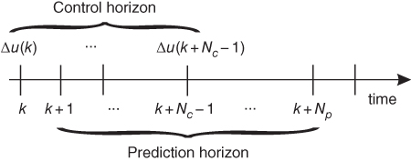
Figure 14.1 Prediction and control horizons.
As presented in Figure 14.1, the prediction horizon must be chosen such that it takes into account the expected effect of the computed control actions in the system. Based on this, the length of the prediction horizon should be at least equal to the length of the control horizon, that is, ![]() . To decrease the computational burden, the lengths should be equal unless the controller is requested to consider changes happening beyond the control horizon.
. To decrease the computational burden, the lengths should be equal unless the controller is requested to consider changes happening beyond the control horizon.
14.3 Control Problem Formulation
The above principle is applied to voltage control and congestion management of DNs. The control variables are the active power (![]() ) and reactive power (
) and reactive power (![]() ) of distributed generators and the voltage set-point of the LTC transformer (
) of distributed generators and the voltage set-point of the LTC transformer (![]() ) at the bulk power supply point, grouped in the
) at the bulk power supply point, grouped in the ![]() vector
vector ![]() , at time
, at time ![]() :
:
where ![]() denotes vector transposition. MPC calculates the control variable changes
denotes vector transposition. MPC calculates the control variable changes ![]() to bring back the monitored branch currents and bus voltages within permissible limits. The controlled variables are directly measured, and grouped in the
to bring back the monitored branch currents and bus voltages within permissible limits. The controlled variables are directly measured, and grouped in the ![]() vector
vector ![]() .1
.1
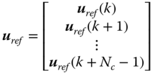
The MPC objective function may be set to minimize the sum of squared control variable changes or the sum of squared deviations between the controls and their references ![]() , as follows:
, as follows:
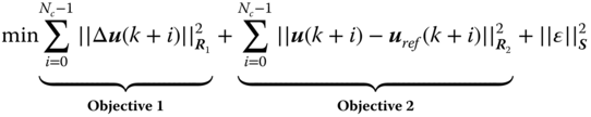
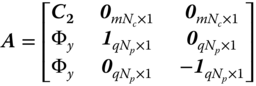
Note that both objectives have been included in (14.2). For the application of concern here, only one will be used depending on what is needed, as will be shown in the following sections. In matrix form, (14.2) can be written as:
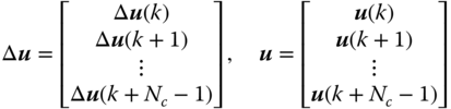
Here, ![]() and
and ![]() are
are ![]()
![]() 1 column vectors defined by:
1 column vectors defined by:
Note that ![]() can be expressed in terms of
can be expressed in terms of ![]() :
:
with
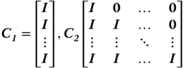
![]() and
and ![]() are the
are the ![]() identity and zero matrices, respectively.
identity and zero matrices, respectively.
Similarly, ![]() is the
is the ![]()
![]() 1 vector of control variable references, which may vary in the control horizon, hence:
1 vector of control variable references, which may vary in the control horizon, hence:
In addition, ![]() is the vector of slack variables used to relax some inequality constraints in case of infeasibility. These variables are heavily penalized by the diagonal matrix
is the vector of slack variables used to relax some inequality constraints in case of infeasibility. These variables are heavily penalized by the diagonal matrix ![]() . Finally,
. Finally, ![]() and
and ![]() are
are ![]() diagonal weighting matrices used to prioritize control actions.
diagonal weighting matrices used to prioritize control actions.
The above objective function is minimized subject to:
where ![]() ,
, ![]() ,
, ![]() , and
, and ![]() are the lower and upper limits on control variables and on their rate of change, along the control horizon. As regards the predicted system evolution, the following equality constraint is also imposed, for
are the lower and upper limits on control variables and on their rate of change, along the control horizon. As regards the predicted system evolution, the following equality constraint is also imposed, for ![]() :
:
where ![]() is the predicted system output at time
is the predicted system output at time ![]() given the measurements at
given the measurements at ![]() , and
, and ![]() is the sensitivity matrix of those variables to control changes.2.
is the sensitivity matrix of those variables to control changes.2.
The last term in (14.10) is included to account for the effect of a known disturbance ![]() in the predicted outputs. Hence,
in the predicted outputs. Hence, ![]() is the sensitivity of those variables to the known disturbance. In addition,
is the sensitivity of those variables to the known disturbance. In addition, ![]() is a binary variable equal to one for the instants when the known disturbance will occur, or zero otherwise.
is a binary variable equal to one for the instants when the known disturbance will occur, or zero otherwise.
The prediction is initialized with ![]() set to the last received measurements. In compact form, (14.10) becomes
set to the last received measurements. In compact form, (14.10) becomes
with,
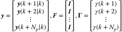
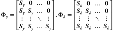
Note that ![]() and
and ![]() are
are ![]() and
and ![]() matrices, respectively.
matrices, respectively.
Finally, the following inequality constraints are imposed to the predicted output:
![]() and
and ![]() are the components of
are the components of ![]() and
and ![]() denotes a
denotes a ![]() unit vector. Additionally,
unit vector. Additionally, ![]() and
and ![]() are the lower and upper allowed output along the prediction horizon:
are the lower and upper allowed output along the prediction horizon:
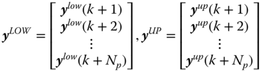
where ![]() and
and ![]() are the minimum and maximum allowed output at time
are the minimum and maximum allowed output at time ![]() .
.
In order to solve the above optimization problem, the equations have to be rearranged into a Quadratic Programming (QP) problem:
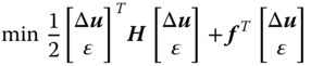
where
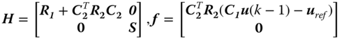
subject to:
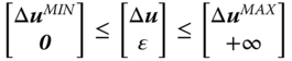
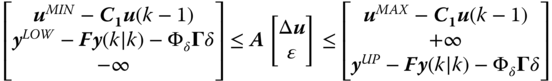
with
![]() is a
is a ![]() null matrix while
null matrix while ![]() and
and ![]() are
are ![]() null and unit matrices.
null and unit matrices.
In the present formulation, there are only two components in ![]() : the first one to relax the lower bound of all controlled variables and the second to relax the upper bound over the prediction horizon. In case of different types of controlled variables, such as bus voltages and branch currents, different slack variables are considered for them (i.e., two for bus voltage and one for branch current limits, see Section 14.5). In this case, matrix
: the first one to relax the lower bound of all controlled variables and the second to relax the upper bound over the prediction horizon. In case of different types of controlled variables, such as bus voltages and branch currents, different slack variables are considered for them (i.e., two for bus voltage and one for branch current limits, see Section 14.5). In this case, matrix ![]() is extended accordingly.
is extended accordingly.
14.4 Voltage Correction With Minimum Control Effort
The first control goal analyzed in this chapter consists of maintaining the DN bus voltages within some predefined limits while minimizing the control deviations, as presented in Objective 1 in (14.2) (with ![]() ).
).
Initially, the operator will define a target voltage for each bus in the network. This target voltage may follow a security or economic purpose, such as network losses minimization. However, trying to reach the actual target values is impractical and likely infeasible. Alternatively, one can try to keep the network voltages within some limits around the target values. In what follows, these limits are referred to as normal operation limits, and the operation within these limits is the controller's main objective.
If any of the bus voltages violate the limits, the controller will use the minimum control actions to bring them within the acceptable limits. As the voltages are in the undesirable region but not in emergency, the controller will use the cheapest controls, since it is not economically justifiable to use expensive controls to maintain voltages in a narrow band of operation. For example, the requested band of operation for a monitored bus voltage may be set at [1.00 1.02] pu. Since the targeted operation might be the result of an OPF, the band might not be the same for all buses. Moreover, the range allowed for each controlled bus may depend on the importance of the customers connected to it or the cost associated with regulating the voltages within a narrow band of operation.
Conversely, if some bus voltages are operating in the unacceptable region, outside some emergency limits, the controller will use all available (both cheap and expensive) actions to return them to the undesirable region. The emergency limits can be the same for all buses. For instance, the operator can define that the network is under emergency conditions if any of the monitored voltages deviates from the range [0.94 1.06] pu. In practice, these limits are defined by the corresponding grid code.

Figure 14.2 Operation states and corrective actions.
Once the controller succeeds in bringing the voltages into the undesirable region, it will again use the cheapest control variables to reach the normal operation conditions.
Figure 14.2 summarizes the transitions between operation states after disturbances and the corresponding corrective actions. Note that there are cases where the correction of some bus voltages is infeasible with the available controls. Under these circumstances, the controller should, at least, apply the control actions that can bring the problematic voltages to a better operating point, even if it is outside the normal operational limits. The controller must do so until a feasible correction is found.
Note that when all voltages lie within the normal operational limits, no control actions are issued, that is, ![]() .
.
14.4.1 Inclusion of LTC Actions as Known Disturbances
A LTC is a slowly acting device that controls the distribution side voltage of the transformer by acting on its turn ratio. The LTC performs a tap change if the controlled voltage remains outside of a dead-band for longer than a predefined delay [20]. This delay is specified to avoid frequent and unnecessary tap changes that may reduce the LTC lifetime. If more than one step is required, the LTC will move by one step at a time with delay between successive moves.
The proposed controller leaves this local control unchanged but acts on the LTC set-point ![]() if appropriate. Therefore, tap changes will be triggered when changes in operating conditions make the controlled voltage
if appropriate. Therefore, tap changes will be triggered when changes in operating conditions make the controlled voltage ![]() leave the dead-band, or when the controller requests a change of
leave the dead-band, or when the controller requests a change of ![]() (and, hence, a shift of the dead-band) such that
(and, hence, a shift of the dead-band) such that ![]() falls outside the dead-band.
falls outside the dead-band.
By assuming that a tap change produces ![]() variation in
variation in ![]() , the number of tap changes can be roughly estimated by:
, the number of tap changes can be roughly estimated by:
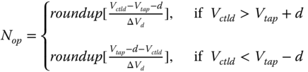
where ![]() is half the LTC dead-band and the function
is half the LTC dead-band and the function ![]() provides the nearest upper integer. Note that
provides the nearest upper integer. Note that ![]() is measurable after an LTC action occurs. This value is assumed constant and it is considered a known value for the controller.
is measurable after an LTC action occurs. This value is assumed constant and it is considered a known value for the controller.
From (14.21), the times of LTC actions can be estimated as:
for ![]() . Here,
. Here, ![]() is the present time instant,
is the present time instant, ![]() is the time delay for the first step, and
is the time delay for the first step, and ![]() is the time delay for subsequent tap steps. The controller can use this information to anticipate the future voltage changes due to the operation of the LTC. In order to do so, the controller must extend the prediction horizon
is the time delay for subsequent tap steps. The controller can use this information to anticipate the future voltage changes due to the operation of the LTC. In order to do so, the controller must extend the prediction horizon ![]() until the last predicted LTC control action is included. A general example of this is provided in Figure 14.3. At instant
until the last predicted LTC control action is included. A general example of this is provided in Figure 14.3. At instant ![]() , it is predicted from (14.21) and (14.22) that three tap changes will take place at
, it is predicted from (14.21) and (14.22) that three tap changes will take place at ![]() ,
, ![]() , and
, and ![]() , respectively, with
, respectively, with ![]() and
and ![]() beyond the control horizon. In order to account for all these LTC actions, the controller extends the prediction horizon up to the smallest discrete time larger than
beyond the control horizon. In order to account for all these LTC actions, the controller extends the prediction horizon up to the smallest discrete time larger than ![]() .
.
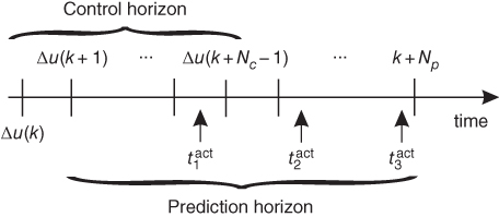
Figure 14.3 Extension of prediction horizon to include predicted LTC actions.
With the controller able to predict the effect of future LTC actions, it is possible to avoid premature and unnecessary output changes of DGUs since it can better decide whether or not the LTC actions are enough to correct the controlled voltages.
14.4.2 Problem Formulation
With the choice of objective function and control variables discussed above, the MPC-based controller has to solve the following QP problem:
subject to:
![]() and
and ![]() are the lower and upper limits of the predicted voltages in
are the lower and upper limits of the predicted voltages in ![]() ; the latter are computed by:
; the latter are computed by:
where ![]() is set to the last received bus voltage measurements,
is set to the last received bus voltage measurements, ![]() contains the sensitivity matrix
contains the sensitivity matrix ![]() of controlled bus voltages to control variables (see (14.13)), and
of controlled bus voltages to control variables (see (14.13)), and ![]() contains the sensitivities of controlled bus voltages to the LTC-controlled voltage (i.e., the last column of matrix
contains the sensitivities of controlled bus voltages to the LTC-controlled voltage (i.e., the last column of matrix ![]() ).
). ![]() is an
is an ![]() vector whose entries are 1 for the instants when the tap changes have been predicted, or 0 otherwise.
vector whose entries are 1 for the instants when the tap changes have been predicted, or 0 otherwise.
The sensitivity of bus voltages with respect to power injections can be obtained off-line from the transposed inverse of the power flow Jacobian matrix [2, 7]. The sensitivities of bus voltages with respect to the LTC-controlled voltage can be approximated by computing the ratio of variations of the monitored bus voltages to the LTC's controlled bus voltage due to a tap change. This information can be easily extracted from the solution of two power flow runs with a single tap position difference. The sensitivity matrix ![]() can be updated infrequently as model errors will be compensated by the MPC scheme [17, 18].
can be updated infrequently as model errors will be compensated by the MPC scheme [17, 18].
The weight assigned to each control variable in ![]() should be related to the cost of the device to provide ancillary services. For example, the reactive power output of a DGU is considered cheaper than its active power output. The latter is actually considered an expensive control action and is not requested unless emergency conditions are encountered. If some of the voltages are outside the emergency limits, the controller will use all controls to correct them. Thus, active powers of DGUs are heavily weighted to minimize their use. Once the voltages reach the undesirable region, only the cheap control variables will be used.
should be related to the cost of the device to provide ancillary services. For example, the reactive power output of a DGU is considered cheaper than its active power output. The latter is actually considered an expensive control action and is not requested unless emergency conditions are encountered. If some of the voltages are outside the emergency limits, the controller will use all controls to correct them. Thus, active powers of DGUs are heavily weighted to minimize their use. Once the voltages reach the undesirable region, only the cheap control variables will be used.
The slack variables ![]() and
and ![]() in (14.26) are used to relax the voltage limits. The entries of the
in (14.26) are used to relax the voltage limits. The entries of the ![]() diagonal matrix
diagonal matrix ![]() should be given very high values.
should be given very high values.
The active power outputs of DGUs are constrained by their capacity. For example, the active power production of conventional synchronous machines is constrained by the turbine capacity. In renewable energy sources, where the production is driven by weather conditions, the corresponding variables of active power are upper bounded by the actual power extracted from the wind or the sun irradiance. This is, at any instant ![]() , the controller cannot request more than the power that is being produced, but it can request active power reductions by partial curtailment. On the other hand, the reactive power output of renewable energy sources is considered fully controllable but subject to capacity limits.
, the controller cannot request more than the power that is being produced, but it can request active power reductions by partial curtailment. On the other hand, the reactive power output of renewable energy sources is considered fully controllable but subject to capacity limits.
Although the maximum reactive power production can be fixed for each DGU, it is desirable to update it with the actual terminal voltage and active power production [21], so that full advantage is taken from its capability. This information is used to update the limits on the control variables.
14.5 Correction of Voltages and Congestion Management with Minimum Deviation from References
The second formulation (Objective 2 in (14.2)) can accommodate various contexts of application, depending on the interactions and information transfers between entities acting on the DGUs, in accordance with regulatory policy. This leads to the definition of a number of operating modes, which are depicted in Figure 14.4.
Besides the monitoring of some bus voltages, active and reactive productions, and terminal voltages of DGUs, this controller variant also monitors the active and reactive power flows in critical (potentially congested) branches. Thus, the controller relies on a dedicated measurement and communication infrastructure but, as suggested in Figure 14.4, it could also rely on the results of a state estimator, for improved system monitoring.
Once the controller observes (or predicts) limit violations, it computes and sends active and/or reactive power corrections to the DGUs of concern. The latter are the differences between the reference and the computed controls, that is:
Note that these corrections should stay at zero as long as no limit violation is observed (or predicted), and come back to zero as soon as operation is no longer constrained, as explained in what follows.
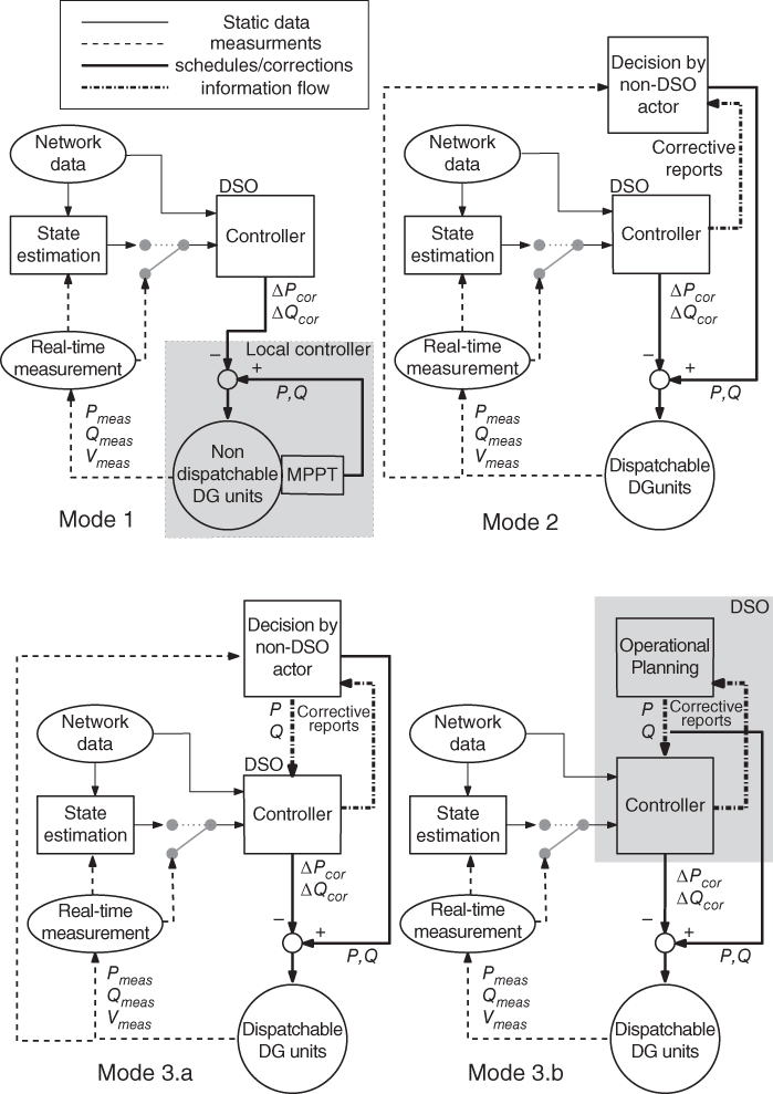
Figure 14.4 Contexts of application of the proposed control scheme.
Furthermore, a distinction is made between dispatchable and non-dispatchable DGUs. The latter are typically wind turbine or photovoltaic units operated for Maximum Power Point Tracking (MPPT). In the absence of operating constraints, they are left to produce as much as can be obtained from the renewable energy source. The dispatchable units, on the other hand, have their production schedules ![]() and
and ![]() , according to market opportunities or balancing needs, for instance.
, according to market opportunities or balancing needs, for instance.
14.5.1 Mode 1
This mode applies to non-dispatchable units. For MPPT purposes, at each time step ![]() , the reference
, the reference ![]() of the
of the ![]() -th DGU should be set to the maximum power available on that unit. This information is likely to be available to the DGU MPPT controller, but is seldom transmitted outside. An alternative is to estimate that power from the measurements
-th DGU should be set to the maximum power available on that unit. This information is likely to be available to the DGU MPPT controller, but is seldom transmitted outside. An alternative is to estimate that power from the measurements ![]() . Considering the short control horizon of concern here, a simple prediction is given by the “persistence” model:
. Considering the short control horizon of concern here, a simple prediction is given by the “persistence” model:
As long as no power correction is applied, the last term is zero and ![]() is used as a short-term prediction of the available power. When a correction is applied, the right-hand side in (14.30) keeps track of what was the available power before a correction started being applied. Using this value as reference allows resetting the DGUs under the desired MPPT mode as soon as system conditions improve.
is used as a short-term prediction of the available power. When a correction is applied, the right-hand side in (14.30) keeps track of what was the available power before a correction started being applied. Using this value as reference allows resetting the DGUs under the desired MPPT mode as soon as system conditions improve.
A more accurate prediction can be used if data are available. That would result in the right-hand side of (14.30) varying with time ![]() .
.
14.5.2 Mode 2
This mode applies to DGUs that are dispatchable but under the control of another actor than the DSO. Thus, the latter does not know the power schedule of the units of concern. In order to avoid interference with that non-DSO actor, the last measured power productions are taken as reference values over the next ![]() time steps:
time steps:
On the other hand, if a control action has been applied by the DSO, to preserve network security, this action should not be counteracted by a subsequent non-DSO action in order to avoid conflict, leading for instance to oscillation. In other words, the DSO is assumed to “have the last word” in terms of corrective actions, since it is the entity responsible for network security.
In both Modes 1 and 2, the controller lacks information to anticipate the DGU power evolution. Hence, the corrections (14.28), (14.29) will be applied ex post, after the measurements have revealed the violation of a (voltage or current) constraint.
14.5.3 Mode 3
This mode relates to dispatchable DGUs whose power schedules are known by the controller, either because this information is transmitted by the non-DSO actors controlling the DGUs (see variant 3.a in Figure 14.4) or because the DSO is entitled to directly control the DGUs (see variant 3.b in Figure 14.4). The latter case may also correspond to schedules determined by DSO operational planning. Unlike in Mode 2, the schedule imposed to the units is known by the controller, which can anticipate a possible violation under the effect of the scheduled change and correct the productions ex ante. Although different from a regulatory viewpoint, Modes 3.a and 3.b are treated in the same way.
Figure 14.5 shows how the ![]() future
future ![]() values are updated with the known schedule before being used as input for the controller. As long as the schedule does not change within the
values are updated with the known schedule before being used as input for the controller. As long as the schedule does not change within the ![]() future time steps (see Figure 14.5a),
future time steps (see Figure 14.5a), ![]() remains unchanged; otherwise, the interpolated values are used.
remains unchanged; otherwise, the interpolated values are used.
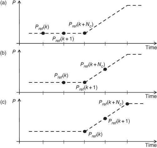
Figure 14.5 Mode 3: updating the  values over three successive times.
In principle, the aforementioned choices also apply to the reference reactive powers ![]() . However, it is quite common to operate DGUs at unity power factor, to minimize internal losses, which amounts to setting
. However, it is quite common to operate DGUs at unity power factor, to minimize internal losses, which amounts to setting ![]() to zero, and corresponds to Mode 3.
to zero, and corresponds to Mode 3.
To make system operation smoother and more secure, the identified limit violations and the corresponding corrections applied by the controller to DGUs should be communicated back to the non-DSO actors or the operational planners, as suggested by the dash-dotted arrows in Figure 14.4.
14.5.4 Problem Formulation
Here the objective is to minimize the sum of squared deviations, over the ![]() future steps, between the controls and their references (i.e., Objective 2 in (14.2)). This leads to the following QP problem, with
future steps, between the controls and their references (i.e., Objective 2 in (14.2)). This leads to the following QP problem, with ![]() in (14.3):
in (14.3):
subject to:
![]() is the upper limit of the predicted currents in
is the upper limit of the predicted currents in ![]() , the latter are computed by:
, the latter are computed by:
where ![]() is set to the last received branch current measurements, and
is set to the last received branch current measurements, and ![]() contains the sensitivity matrix
contains the sensitivity matrix ![]() of controlled branch currents to control variables.
of controlled branch currents to control variables.
The sensitivity matrix ![]() should be updated more frequently, due to the higher variability of currents. The sensitivity of the branch current
should be updated more frequently, due to the higher variability of currents. The sensitivity of the branch current ![]() with respect to the
with respect to the ![]() -th DGU active (resp. reactive) power
-th DGU active (resp. reactive) power ![]() (resp.
(resp. ![]() ) can be obtained as [4]:
) can be obtained as [4]:
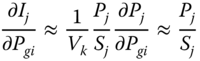
where ![]() ,
, ![]() , and
, and ![]() are respectively the active, reactive, and apparent power flows in the branch, and
are respectively the active, reactive, and apparent power flows in the branch, and ![]() is the voltage at the bus where the current is measured. The voltage is simply taken equal to 1 pu. The above approximations assume that
is the voltage at the bus where the current is measured. The voltage is simply taken equal to 1 pu. The above approximations assume that ![]() (resp.
(resp. ![]() ) does not change much when
) does not change much when ![]() (resp.
(resp. ![]() ) is varied, and the change of
) is varied, and the change of ![]() (resp.
(resp. ![]() ) is equal to the change in
) is equal to the change in ![]() (resp.
(resp. ![]() ). Note that this approximation applies only if the
). Note that this approximation applies only if the ![]() -th branch is on the path from the
-th branch is on the path from the ![]() -th DGU to the HV/MV tranformer; otherwise, a zero sensitivity is assumed since the branch current would not change with the DGU power change. Note also that using (14.38) and (14.39) requires having the branch equipped with active and reactive power flow measurements.
-th DGU to the HV/MV tranformer; otherwise, a zero sensitivity is assumed since the branch current would not change with the DGU power change. Note also that using (14.38) and (14.39) requires having the branch equipped with active and reactive power flow measurements.
In this formulation, ![]() should be updated at each discrete step while
should be updated at each discrete step while ![]() may be kept constant at all operating points.
may be kept constant at all operating points.
The diagonal weighting matrix ![]() allows prioritizing the controls, with lower values assigned to reactive than to active power deviations. Unlike the former formulation, DGU active power may be requested to change in undesirable conditions, not only in an emergency.
allows prioritizing the controls, with lower values assigned to reactive than to active power deviations. Unlike the former formulation, DGU active power may be requested to change in undesirable conditions, not only in an emergency.
The new slack variable ![]() is used to relax (14.36) in case of infeasibility; the entries of the
is used to relax (14.36) in case of infeasibility; the entries of the ![]() diagonal matrix
diagonal matrix ![]() are given very high values.
are given very high values.
To obtain a smooth system evolution, the bounds ![]() ,
, ![]() and
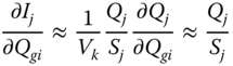
and ![]() on the predicted voltages and currents are tightened progressively. An exponential evolution with time has been considered, as shown in Figure 14.6 for respectively a lower voltage (Figure 14.6a) and a current limit (Figure 14.6b). The circles indicate voltage or current values measured at time
on the predicted voltages and currents are tightened progressively. An exponential evolution with time has been considered, as shown in Figure 14.6 for respectively a lower voltage (Figure 14.6a) and a current limit (Figure 14.6b). The circles indicate voltage or current values measured at time ![]() , which fall outside the acceptable range. The limits imposed at the successive times
, which fall outside the acceptable range. The limits imposed at the successive times ![]() are shown with solid lines. They force the voltage or current of concern to enter the acceptable range at the end of the prediction horizon. Taking the lower voltage limit as an example, the variation is given by
are shown with solid lines. They force the voltage or current of concern to enter the acceptable range at the end of the prediction horizon. Taking the lower voltage limit as an example, the variation is given by ![]() :
:
where ![]() is the bus of concern,
is the bus of concern, ![]() is a smoothing time constant and
is a smoothing time constant and ![]() is the measurement received at time
is the measurement received at time ![]() . If it does not exceed the desired limit, that is, if
. If it does not exceed the desired limit, that is, if ![]() , the latter is used as constant bound in (14.35), at all future times, that is,
, the latter is used as constant bound in (14.35), at all future times, that is, ![]() .
.
Similar variations are considered for the upper voltage and the current limits. As regards the latter, the ![]() value is set conservatively below the effective thermal capability monitored by the corresponding protection, as shown in Figure 14.6b.
value is set conservatively below the effective thermal capability monitored by the corresponding protection, as shown in Figure 14.6b.
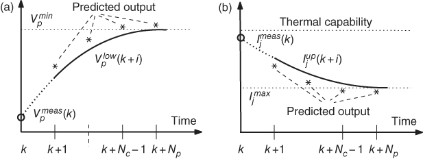
Figure 14.6 Progressive tightening of voltage and current bounds.
14.6 Test System
The multi-step receding-horizon controllers presented above have been tested through simulations of a 75-bus, 11-kV radial DN hosting 22 DGUs; the line parameters are available in [22] and the network topology is shown in Figure 14.7.
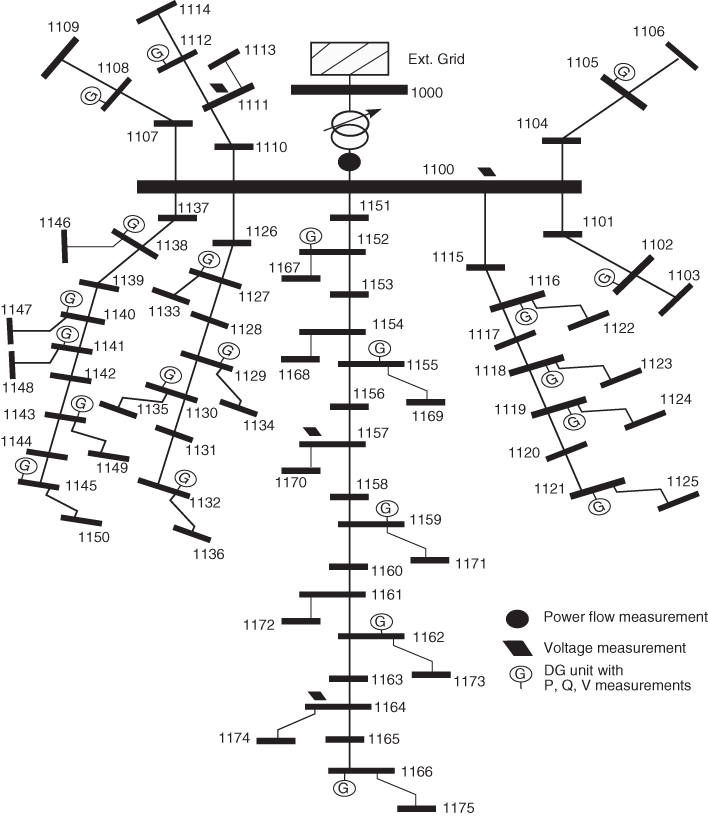
Figure 14.7 Network topology and measurement allocation.
The distribution system is connected to the external grid through a 33/11 kV transformer equipped with an LTC. The network topology consists of 8 feeders all directly connected to the main transformer, and they serve 38 loads modeled as constant current for active power and constant impedance for reactive power, and 15 more loads represented by equivalent induction motors.
In this test system, 13 out of the 22 DGUs are 3-MVA synchronous generators driven by hydro turbines with 2.55 MW of maximum capacity. The remaining nine DGUs are Doubly-Fed Induction Generators (DFIG) driven by wind turbines. Each DFIG is a one-machine equivalent of two 1.5 MW wind turbines operating in parallel. The nominal capacity of each DFIG is 3.33 MVA. The model of the wind turbine and its parameters were taken from [23].
The DFIGs operate in reactive power control mode. This is achieved by a PI controller that regulates the reactive power output according to the set-point value requested by the centralized controller. Compared to the synchronous machines, this reactive power control loop has a faster response.
The reactive power limits of DGUs are calculated, at any time ![]() , given their actual operation conditions (
, given their actual operation conditions (![]() and
and ![]() ) and their nominal capacities [21]. Hence, any reactive power increase requested by the controller will not compromise the DGUs' active power output or violate the machine capacities.
) and their nominal capacities [21]. Hence, any reactive power increase requested by the controller will not compromise the DGUs' active power output or violate the machine capacities.
It is assumed that the 22 DGUs are allocated with remote units that measure the active power, reactive power, and voltage magnitude at their terminals. These measurements are used by the centralized controller.
As regards load buses, the measurement configuration is such that no load is at a distance larger than two buses from a voltage monitored bus (see Figure 14.7). By following this rule, there are three load buses with monitored voltages. These voltage measurements along with the power output measurement of the DGUs make up a set of 71 measurements received by the controller.
It is not possible to ensure that non-monitored voltages will be within the desirable limits. However, by distributing the measurements all over the network, it is reasonable to expect that the voltages of non-monitored buses will be close to the voltages of the neighboring controlled buses.
The measurements are collected some time after the control actions are applied. This is to wait for the system response and to avoid making decisions based on measurements taken during transients.
Because of the fast sampling rate of modern monitoring units and their efficient communication links, it is assumed that the measurements are collected every 0.2![]() .
.
The measurements were simulated by adding white Gaussian noise restricted to ![]() for
for ![]() measurements and
measurements and ![]() of the respective DGU maximum power output for
of the respective DGU maximum power output for ![]() and
and ![]() measurements. In order to filter out some of this noise, the controller uses the average of the 11 snapshots received over a time window of 2 s.
measurements. In order to filter out some of this noise, the controller uses the average of the 11 snapshots received over a time window of 2 s.
The controller sends corrections every 10 s. The prediction and control horizons are set to ![]() . This yields a good compromise between sufficient number of MPC steps and a short enough response time to correct violations.
. This yields a good compromise between sufficient number of MPC steps and a short enough response time to correct violations.
It must be emphasized that the changes in operating point applied to the system, such as wind variations, load increases, and scheduled changes, have been made faster than in reality for a legible presentation of the results.
14.7 Simulation Results: Voltage Correction with Minimal Control Effort
In the first two scenarios (A and B), it is required that the monitored voltages remain within the [1.000 1.025] pu range while minimizing (14.23). In addition, the system is considered under emergency conditions when any bus reaches voltages outside the [0.940 1.060] pu interval.
The active and reactive power of DGUs are not allowed to change by more than 0.5 MW and 0.5 MVar respectively, while the LTC set-point is not allowed to change more than 0.01 pu per discrete time step.
In the objective function (14.23), identical costs have been assumed for all DGUs. Changes of the reactive power outputs cost the same as changes in LTC voltage set-point while the cost for active power changes is set 10 times higher. Moreover, the cost of using the slack variables is 1000 times higher than that of reactive power.
Since the variation of load powers with voltage are not well known in practice, the sensitivity matrix has been calculated by considering constant power models for all loads. In addition, the line parameters used to calculate the sensitivity matrix were corrupted by a random error whose mean value is zero and standard deviation is ![]() of the actual line parameter. The objective is to demonstrate that the controller is robust and can compensate for these model inaccuracies.
of the actual line parameter. The objective is to demonstrate that the controller is robust and can compensate for these model inaccuracies.
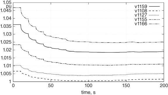
Figure 14.8 Scenario A: Voltage correction.
14.7.1 Scenario A
The first scenario reported consists of the presence of over voltages in certain areas of the network caused by low power demands and high power production from DGUs. With the available set of measurements, it is found that the voltages in some areas are outside the normal operation constraints, but not enough to reach the emergency state. Here it is pointed out that, for legibility purposes, the following plots show the exact (noiseless) voltages and DGU power outputs, as opposed to the noisy and discrete measurements received and processed by the controller.
Figure 14.8 presents the obtained correction of the voltages starting at ![]() = 10 s and changing every 10 s thereafter, under the effect of the controller adjusting the DGU reactive powers. Note that the controller yields an exponentially decreasing correction of the bus voltages until the latter reach the desired interval.
= 10 s and changing every 10 s thereafter, under the effect of the controller adjusting the DGU reactive powers. Note that the controller yields an exponentially decreasing correction of the bus voltages until the latter reach the desired interval.
The selected curves in Figure 14.8, correspond to the most representative voltages in the network. The only load bus voltage reported is v1159 whereas the remaining voltages correspond to DGU buses.
Although most of the DGUs reduced their reactive power production, the ones connected to buses 1102 and 1108 were requested to increase (see Figure 14.9). This is because the controller anticipated that the voltages near bus 1108 would violate the lower limit of 1 pu. Hence, the reactive powers of these machines increase to maintain those voltages within limits.
From Figure 14.9 it is seen that the maximum change of reactive power output occurs in the DGU at bus 1166. This machine is requested to absorb reactive power until the most problematic voltage v1166 is corrected.
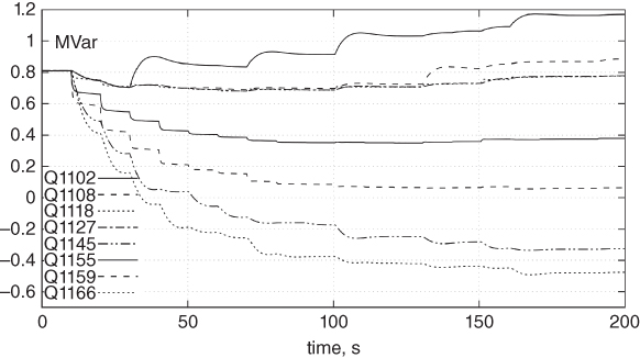
Figure 14.9 Scenario A: Reactive power output of the DGUs.
As soon as all the monitored voltages are brought back inside the limits, the controller does not request further changes in ![]() . This condition is met at
. This condition is met at ![]() = 190 s. These results confirm that even in the presence of inaccurate sensitivity values, the controller is able to correct the voltages.
= 190 s. These results confirm that even in the presence of inaccurate sensitivity values, the controller is able to correct the voltages.
14.7.2 Scenario B
The second scenario reported consists of an external voltage drop that affects the voltages at all buses. This disturbance was simulated by a negative step change of 0.08 pu of the Thévenin equivalent voltage, at the primary side of the main transformer. For this case, the LTC is coordinated along with the DGUs to correct the voltage drop in the DN. The purpose of this test is to demonstrate the prediction capability of the proposed controller and how this avoids unnecessary changes of alternative controls.
Figure 14.10 presents the voltage correction at a sample of monitored buses. The problem is corrected at about 90 s after the operation of the LTC and a few changes of the DGU power outputs. Just after the disturbance at ![]() s, the difference between
s, the difference between ![]() and its set-point is enough to trigger eight tap movements (see (14.21)). The first tap operation occurs at
and its set-point is enough to trigger eight tap movements (see (14.21)). The first tap operation occurs at ![]() s and the subsequent ones occur in steps of 10 s until
s and the subsequent ones occur in steps of 10 s until ![]() s. After this time, no more LTC actions are required.
s. After this time, no more LTC actions are required.
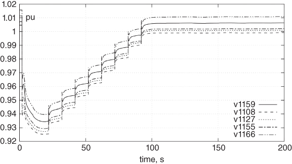
Figure 14.10 Scenario B: Voltage correction.
The tiny voltage corrections seen mainly at bus 1166 at ![]() s and
s and ![]() s were triggered by the noise affecting voltage measurements that indicated small violations of the monitored voltages.
s were triggered by the noise affecting voltage measurements that indicated small violations of the monitored voltages.
Table 14.1 details the future tap movements as anticipated by the controller. Equations 14.21 and 14.22 are used for this purpose. It is found that the LTC will operate seven times. The controller makes a rough estimate of the LTC time actions. For example, it wrongly anticipated that the first LTC action would occur at ![]() s, while it actually occurred at
s, while it actually occurred at ![]() s. This example confirms that there is no need to know the exact moment at which the LTC will act. In fact, any mistake in prediction will be corrected and updated when new measurements are available. The important aspect is that the controller can anticipate future actions and use this information to avoid more expensive control actions.
s. This example confirms that there is no need to know the exact moment at which the LTC will act. In fact, any mistake in prediction will be corrected and updated when new measurements are available. The important aspect is that the controller can anticipate future actions and use this information to avoid more expensive control actions.
Table 14.1 Controller Anticipation of the LTC Actions
| 10 | 7 | 9 | 30 | 40 | 50 | 60 | 70 | 80 | 90 |
| 20 | 7 | 8 | 30 | 40 | 50 | 60 | 70 | 80 | 90 |
| 30 | 7 | 7 | 30 | 40 | 50 | 60 | 70 | 80 | 90 |
| 40 | 6 | 6 | 40 | 50 | 60 | 70 | 80 | 90 | − |
| 50 | 5 | 5 | 50 | 60 | 70 | 80 | 90 | − | − |
| 60 | 3 | 3 | 60 | 70 | 80 | − | − | − | − |
| 70 | 3 | 3 | 70 | 80 | 90 | − | − | − | − |
| 80 | 2 | 3 | 80 | 90 | − | − | − | − | − |
| 90 | 1 | 3 | 90 | − | − | − | − | − | − |
In order to capture all the anticipated future events due to LTC actions, the controller extended its prediction horizon length. For example, at ![]() s, the controller anticipated that the last control action would occur at
s, the controller anticipated that the last control action would occur at ![]() s. Hence, it automatically increases
s. Hence, it automatically increases ![]() from three to nine steps. For
from three to nine steps. For ![]() s,
s, ![]() is reset to three.
is reset to three.
Figure 14.11 presents the coordinated reactive power output of the DGUs. Since the controller is able to predict the effect of the LTC's future actions in the controlled voltages, it did not require significant changes of ![]() . A similar behavior occurs for changes in active power outputs during emergency conditions. One could argue that there is a cost associated with many tap movements due to wear of equipment. This could be included in the cost function to reduce the number of tap changes by making use of other available control variables.
. A similar behavior occurs for changes in active power outputs during emergency conditions. One could argue that there is a cost associated with many tap movements due to wear of equipment. This could be included in the cost function to reduce the number of tap changes by making use of other available control variables.
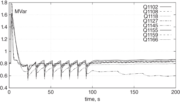
Figure 14.11 Scenario B: Reactive power output of the DGUs.
14.8 Simulation Results: Voltage and/or Congestion Corrections with Minimum Deviation from Reference
The last three scenarios reported in this section evaluate the control scheme presented in Section 14.5. The matrices ![]() and
and ![]() are diagonal with entries equal to 1 for reactive powers, 25 for active powers, 500 for the slack variables
are diagonal with entries equal to 1 for reactive powers, 25 for active powers, 500 for the slack variables ![]() and
and ![]() , and 5000 for
, and 5000 for ![]() . In addition, only the power output of DGUs are considered control variables.
. In addition, only the power output of DGUs are considered control variables.
14.8.1 Scenario C: Mode 1
All 22 DGUs are assumed to be driven by wind turbines, operated for MPPT. Thus the control of all DGUs is in Mode 1 (see Figure 14.4). Initially, the dispersed generation exceeds the load, and the DN is injecting active power into the external grid. At the same time, the DGUs are operating at unity power factor, and the DN draws reactive power from the external grid.
A 10% increase in wind speed takes place from ![]() to
to ![]() s, as shown in Figure 14.12. This results in an increase of the active power flow in the transformer, as shown in Figure 14.13. At
s, as shown in Figure 14.12. This results in an increase of the active power flow in the transformer, as shown in Figure 14.13. At ![]() s, the thermal limit of the latter, shown with heavy line in Figure 14.13, is exceeded. This is detected by the controller through a violation of the constraint (14.36) at
s, the thermal limit of the latter, shown with heavy line in Figure 14.13, is exceeded. This is detected by the controller through a violation of the constraint (14.36) at ![]() s.
s.
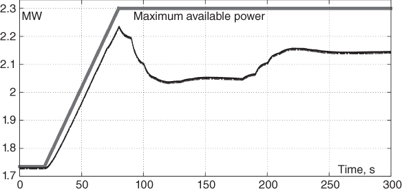
Figure 14.12 Scenario C: Active power produced by DGUs.
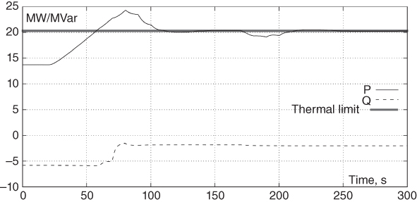
Figure 14.13 Scenario C: Power flows in the transformer.
The controller corrects this congestion problem by acting first on the DGU reactive powers, which have higher priority through the weighting factors. Figure 14.14 shows that the controller makes some DGUs produce reactive power, to decrease the import (and, hence, the current) through the transformer. The latter effect can be seen in Figure 14.13. However, the correction of DGU reactive powers alone cannot alleviate the overload, and from ![]() s on, the controller curtails the active power of wind turbines as shown by Figure 14.12. The overload is fully corrected at
s on, the controller curtails the active power of wind turbines as shown by Figure 14.12. The overload is fully corrected at ![]() s.
s.
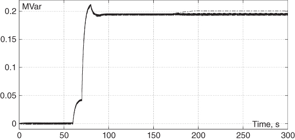
Figure 14.14 Scenario C: Reactive power produced by DGUs.
To illustrate the ability of the proposed control scheme to steer the DGUs back to MPPT, the system operating conditions are relieved by simulating a 4.1 MW load increase starting at ![]() s. The corresponding decrease of the active power flow in the transformer can be observed in Figure 14.13. This leaves some space to restore part of the curtailed DGU active powers. As expected, the controller increases the DGU productions until the transformer current again reaches its limit, at around
s. The corresponding decrease of the active power flow in the transformer can be observed in Figure 14.13. This leaves some space to restore part of the curtailed DGU active powers. As expected, the controller increases the DGU productions until the transformer current again reaches its limit, at around ![]() s. Figure 14.12 shows that, indeed, the active productions get closer to the maximum power available from wind.
s. Figure 14.12 shows that, indeed, the active productions get closer to the maximum power available from wind.
The unpredicted thermal limit violation caused by the initial wind increase was corrected ex post. It is interesting to note that, on the contrary, when taking advantage of the load relief, the controller steers the system in such a way that it does not exceed the thermal limit.
14.8.2 Scenario D: Modes 1 and 2 Combined
It is now assumed that nine units, connected to buses 1118, 1119, 1129, 1132, 1138, 1141, 1155, 1159, and 1162 (see Figure 14.7), are driven by wind turbines and are non-dispatchable. They are thus operated in Mode 1. However, since the wind speed is assumed constant in this scenario, the productions of those units remain constant.
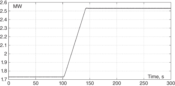
Figure 14.15 Scenario D: Active power produced by dispatchable units.
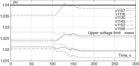
Figure 14.16 Scenario D: Bus voltages.
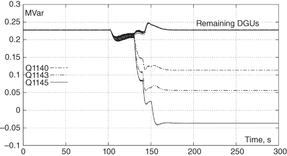
Figure 14.17 Scenario D: Reactive power produced by dispatchable units.
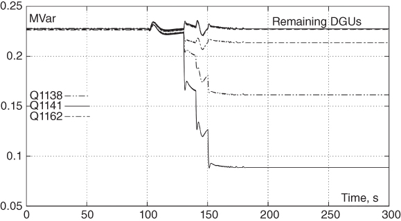
Figure 14.18 Scenario D: Reactive power produced by non-dispatchable units.
The remaining 13 DGUs use synchronous generators and are dispatchable. They are operated in Mode 2. An increase of their active power by an actor other than the DSO, thus not known by the controller, takes place from ![]() to
to ![]() s, as shown in Figure 14.15. The schedule leaves the reactive powers unchanged. Since the initial network voltages are close to the admissible upper limit, shown by the heavy line in Figure 14.16, the system experiences high voltage problems.
s, as shown in Figure 14.15. The schedule leaves the reactive powers unchanged. Since the initial network voltages are close to the admissible upper limit, shown by the heavy line in Figure 14.16, the system experiences high voltage problems.
The controller does not send corrections until ![]() s, when the voltage at bus 1145 exceeds the limit. Over the 40 seconds that follow this limit violation, the controller adjusts the reactive powers of both dispatchable and non-dispatchable units, as shown by Figures 14.17 and 14.18. It is easily seen that different corrections are applied to different DGUs, depending on their locations in the system. It is also seen from Figure 14.16 that the voltage at bus 1145 crosses the limit several times, followed by reactive power adjustments. These ex post corrections were to be expected since, in this example, the DGUs are either in Mode 1 or in Mode 2.
s, when the voltage at bus 1145 exceeds the limit. Over the 40 seconds that follow this limit violation, the controller adjusts the reactive powers of both dispatchable and non-dispatchable units, as shown by Figures 14.17 and 14.18. It is easily seen that different corrections are applied to different DGUs, depending on their locations in the system. It is also seen from Figure 14.16 that the voltage at bus 1145 crosses the limit several times, followed by reactive power adjustments. These ex post corrections were to be expected since, in this example, the DGUs are either in Mode 1 or in Mode 2.
14.8.3 Scenario E: Modes 1 and 3 Combined
In this last scenario, some DGUs are non dispatchable and operated in Mode 1, while the dispatchable ones are operated in Mode 3, with their schedules known by the controller. The latter may come, for instance, from operational planning decisions.
Two successive changes of DGU active powers are considered: (i) an unforeseen wind speed change from ![]() to
to ![]() s increasing the production of the non-dispatchable units, and (ii) a power increase of the dispatchable units scheduled to take place from
s increasing the production of the non-dispatchable units, and (ii) a power increase of the dispatchable units scheduled to take place from ![]() to
to ![]() s. The corresponding active power generations are shown in Figure 14.19.
s. The corresponding active power generations are shown in Figure 14.19.
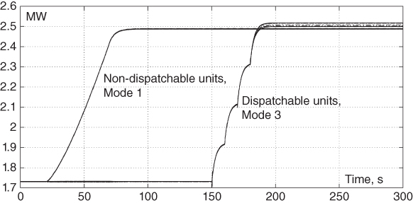
Figure 14.19 Scenario E: Active power produced by various units.
Figure 14.20 shows the resulting evolution of a few bus voltages. The increase in wind power makes them approach their limit, shown by the heavy line. Without a corrective action, the subsequent scheduled change would cause a limit violation. However, the latter change is anticipated by the controller, through the ![]() values updated as shown in Figure 14.5. Therefore, the controller anticipatively adjusts the DGU reactive powers, as seen in Figures 14.21 and 14.22, and no voltage exceeds the limit while all the active power changes are accommodated. The controller anticipative behavior is clearly seen in Figure 14.20, where the voltage decrease resulting from the reactive power adjustment counteracts the increase due to active power increase, leading the highest voltage to land on the upper limit.
values updated as shown in Figure 14.5. Therefore, the controller anticipatively adjusts the DGU reactive powers, as seen in Figures 14.21 and 14.22, and no voltage exceeds the limit while all the active power changes are accommodated. The controller anticipative behavior is clearly seen in Figure 14.20, where the voltage decrease resulting from the reactive power adjustment counteracts the increase due to active power increase, leading the highest voltage to land on the upper limit.
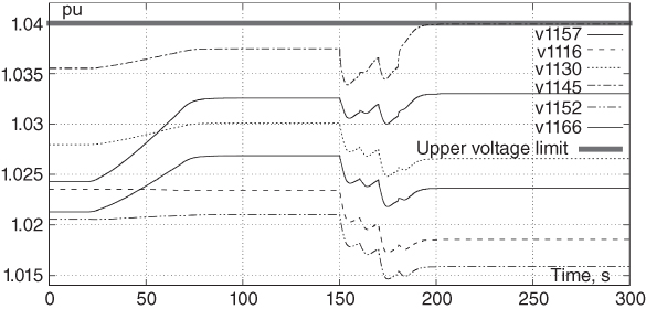
Figure 14.20 Scenario E: Bus voltages.
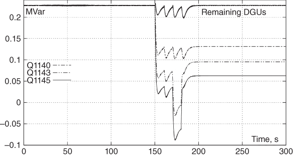
Figure 14.21 Scenario E: Reactive power produced by dispatchable units.
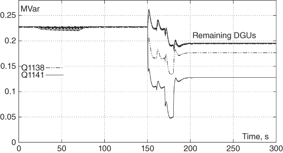
Figure 14.22 Scenario E: Reactive power produced by non-dispatchable units.
14.9 Conclusion
This chapter has presented a scheme for corrective control of voltages and congestion management of DNs based on MPC. It is demonstrated how temporary abnormal conditions can be overcome with a correct selection of DGU power outputs.
The main features of the MPC-based scheme are recalled hereafter:
- Bus voltages and branch currents are controlled such that they remain within an acceptable range of operation. Hence, the controllers do not act unless these limits are violated or the reference values of productions have been changed.
- The controllers discriminate between cheap and expensive control actions and can select the appropriate set of control variables depending on the regions of operation.
- Being based on multiple time step optimization, these controllers are able to smoothly drive the system from its current to the targeted operation region.
- Due to the closed-loop nature of MPC, the control schemes can compensate for model inaccuracies and failure or delays of the control actions.
- Lastly, owing to their anticipation capabilities, these controllers also take into consideration the requested actions that will be applied in the future. This is a common situation when the LTC of the transformer is requested to operate at time
 but acts later due to standard control delays. Accounting for future control actions avoids the premature and maybe unnecessary dispatch of other control actions.
Thanks to the repeated computations, MPC offers some inherent fault-tolerance capability (particularly with respect to modeling errors and control failure). Illustrative examples pertaining to voltage control can be found in [3, 13]. The fault-tolerance can be further increased if the MPC is supported by an intelligent fault identification and detection scheme. With this support, even re-configurable control can be achieved [12].
Improved modeling could deal with the dynamic response of the controlled devices. The DGUs considered in this chapter relate to power-electronics interfaces and, hence, were assumed to react faster than the MPC sampling period of—typically—10 seconds. This justifies using a static representation, through sensitivity matrices, to predict the future system evolution. Dynamic models would be required for slower responding devices or if the MPC sampling period was decreased. It has also been suggested that artificial neural networks could be a viable option to further enhance MPC performance [12].
References
- 1 Q. Gemine, E. Karangelos, D.E. and Cornelusse, B. (2013) Active network management: planning under uncertainty for exploiting load modulation, in IREP Symposium-Bulk Power System Dynamics and Control -IX, Rethymnon, Greece.
- 2 Borghetti, A., Bosetti, M., Grillo, S., Massucco, S., Nucci, C., Paolone, M., and Silvestro, F. (2010) Short-term scheduling and control of active distribution systems with high penetration of renewable resources. IEEE Systems Journal, 4 (3), 313–322.
- 3 Valverde, G. and Van Cutsem, T. (2013) Control of dispersed generation to regulate distribution and support transmission voltages, in Proceedings of IEEE PES 2013 PowerTech conference.
- 4 Soleimani Bidgoli, H., Glavic, M., and Van Cutsem, T. (2014) Model predictive control of congestion and voltage problems in active distribution networks, in Proc. CIRED conference, paper No 0108.
- 5 Vovos, P.N., Kiprakis, A.E., Wallace, A.R., and Harrison, G.P. (2007) Centralized and distributed voltage control: Impact on distributed generation penetration. IEEE Transactions on Power Systems, 22 (1), 476–483.
- 6 Dolan, M., Davidson, E., Kockar, I., Ault, G., and McArthur, S. (2012) Distribution power flow management utilizing an online optimal power flow technique. IEEE Transactions on Power Systems, 27 (2), 790–799.
- 7 Zhou, Q. and Bialek, J. (2007) Generation curtailment to manage voltage constraints in distribution networks. IET Generation Transmission and Distribution, 1 (3), 492–498.
- 8 Sansawatt, T., Ochoa, L.F., and Harrison, G.P. (2012) Smart decentralized control of DG for voltage and thermal constraint management. IEEE Transactions on Power Systems, 27 (3), 1637–1645.
- 9 Hambrick, J. and Broadwater, R.P. (2011) Configurable, hierarchical, model-based control of electrical distribution circuits. IEEE Transactions on Power Systems, 26 (3), 1072–1079.
- 10 Leisse, I., Samuelsson, Q., and Svensson, J. (2013) Coordinated voltage control in medium and low voltage distribution networks with wind power and photovoltaics, in IEEE PES PowerTech Conference, Grenoble, p. 6.
- 11 Degefa, M., Lehtonen, M., Millar, R., Alahäivälä, A., and Saarijärvi, E. (2015) Optimal voltage control strategies for day-ahead active distribution network operation. Electric Power Systems Research, 127, 41–52.
- 12 Maciejowski, J.M. (2002) Predictive Control With Constraints, Prentice-Hall.
- 13 Glavic, M., Hajian, M., Rosehart, W., and Van Cutsem, T. (2011) Receding-horizon multi-step optimization to correct nonviable or unstable transmission voltages. IEEE Transactions on Power Systems, 26 (3), 1641–1650.
- 14 Qin, S. and Badgwell, T.a. (2003) A survey of industrial model predictive control technology. Control Engineering Practice, 11 (7), 733–764.
- 15 Farina, M., Guagliardi, A., Mariani, F., Sandroni, C., and Scattolini, R. (2015) Model predictive control of voltage profiles in MV networks with distributed generation. Control Engineering Practice, 34, 18–29.
- 16 Falahi, M., Lotfifard, S., Ehsani, M., and Butler-Purry, K. (2013) Dynamic model predictive-based energy management of DG integrated distribution systems. IEEE Transactions on Power Delivery, 28 (4), 2217–2227.
- 17 Valverde, G. and Van Cutsem, T. (2013) Model predictive control of voltages in active distribution networks. IEEE Transactions on Smart Grid, 4 (4), 2152–2161.
- 18 Soleimani Bidgoli, H., Glavic, M., and Van Cutsem, T. (2016) Receding-horizon control of distributed generation to correct voltage or thermal violations and track desired schedules, in Proc. 19th Power Systems Computation Conference (PSCC), Genoa, Paper. No. 114, p. 7.
- 19 Bemporad, A. and Morari, M. (1999) Robust model predictive control: A survey. Robustness in identification and control, 245, 207–226.
- 20 Van Cutsem, T. and Vournas, C. (1998) Voltage Stability of Electric Power Systems, Springer.
- 21 Valverde, G. and Orozco, J. (2014) Reactive power limits in distributed generators from generic capability curves, in Proc. IEEE PES 2014 General Meeting, Washington DC., p. 5.
- 22 Centre for Sustainable Electricity and Distributed Generation, United Kingdom Generic Distribution Network, available online: https://github.com/sedg/ukgds.
- 23 G. Tsourakis, B.N. and Vournas, C. (2009) Effect of wind parks with doubly fed asynchronous generators on small-signal stability. Electrical Power System Research, 79 (1), 190–200.