Chapter 9
Model-based Predictive Control for Damping Electromechanical Oscillations in Power Systems
Da Wang
Researcher of Intelligent Electrical Power Systems, Intelligent Electrical Power Grids (IEPG), TU Delft, Netherlands
9.1 Introduction
Electromechanical oscillations mean relative motions of generator shafts and resultant fluctuations of electrical variables (current, voltage, etc.) In modern large-scale electrical power systems, long transmission distances over weak grids, highly variable generation patterns, heavy loading, and so on, tend to increase the probability of appearance of sustained wide area electromechanical oscillations [1, 2]. Moreover, higher and higher penetration of renewable energy also changes current damping characteristics and increases the risk of oscillation instability [3]. Such oscillations threaten the security of power systems, and if they cause cascading faults, can lead to large-scale blackouts [4].
It is usually considered that electromechanical oscillations are caused by insufficient damping of power systems. Consequently, most researches on damping oscillations focus on developing different controllers, like Power System Stabilizers (PSSs), and Thyristor Controlled Series Compensators (TCSCs), in order to improve system damping [5]. Conventionally, these controllers use local measurements at their inputs. The control rules are determined in off-line studies using time domain simulations such as Prony or Eigen analysis, and remain fixed in practice. With recent developments in Wide Area Measurement Systems (WAMSs), further research is being devoted to improving the ability to damp inter-area oscillations by introducing global signals [6, 7].
Indeed, the damping depends on the structure, controller setting, and operation mode of power systems, but the latter continuously varies in practice. Therefore, an expected damping controller should first be able to adaptively adjust its control behaviors following changes of operation conditions. Moreover, since global damping effects are decided by all damping controllers scattered into different areas and installed at different times, a good damping controller is also expected to coordinate with other controllers in order to obtain satisfactory global effects.
Based on advances in power system modeling and large-scale optimization, a new idea is to apply Model Predictive Control (MPC) to design such an adaptive and coordinated damping controller. MPC is a proven technique with numerous real-life applications, whose success comes from three factors: an explicit process model, a future temporal horizon, and an ability to deal with different constraints [8, 9]. These factors allow MPC to deal with all significant dynamics over a future temporal horizon and to drive the outputs of the controlled plant to evolve more closely along a desired trajectory, under the condition of satisfying different constraints on inputs, states, and outputs.
MPC has been applied to optimal power flow, voltage regulation, and dynamic stability of power systems [10–12]. As far as damping control of electromechanical oscillations is concerned, one of the earliest MPC applications is presented in [13] where generalized predictive control is used to switch capacitors. The control strategy is computed by minimizing a quadratic cost function that combines local system outputs and rates-of-change of controls over a prediction horizon. An MPC for step-wise series reactance modulation of a TCSC is presented in [14] to stabilize electromechanical oscillations, where a reduced two-machine model of the power system is used and updated using local measurements. Penalizing deviations of predicted outputs and control increments through an objective function, reference [15] proposes a model predictive adaptive controller to damp inter-area oscillations in a four-generator system. In references [16, 17], a bank of linearized system models is developed to represent system response under oscillations. For each model in the bank, an observer-based state feedback controller is designed a priori, and MPC optimizes the weights for individual controllers.
In this chapter, MPC is applied to calculate supplementary signals for existing damping controllers (exciters and TCSC). These signals are superimposed on the inputs of controllers and continuously updated in order to improve and coordinate the damping effects of the controllers. Defining angular speeds as outputs, MPC treats damping control as a multi-step optimization problem with discrete dynamics and costs, which penalizes deviations of angular speeds from the reference speed over a future horizon. At each control time, MPC collects current system states, solves this optimization problem, and calculates supplementary signals. Utilizing these signals, it forces angular speeds to return to the reference speed and remain as close to the latter as possible. When all generators are running at the reference speed, oscillations are damped.
In order to implement this idea, a centralized MPC controller is first designed based on a linearized, discrete state space model. Its performance is evaluated both in ideal conditions and considering realistic State Estimation (SE) errors and computation and communication delays. Different damping controllers are also studied in order to assess their versatility. Next, the centralized MPC is further extended into a distributed one with the aim of making it more viable for large-scale or multi-area systems. The decoupling and coordination between subsystems is analyzed. Finally, a robust hierarchical MPC is proposed that introduces a second layer of MPC controllers on local generators. The performances of three MPC schemes are demonstrated and compared on a 16-generator, 70-bus system.
9.2 MPC Basic Theory & Damping Controller Models
9.2.1 What is MPC?
The basic idea of MPC is illustrated in Figure 9.1, which describes dynamic control of a single-input single-output system [18]. System dynamics are discretized by a small simulation step of δ seconds. Every Δt seconds, MPC is carried out one time. It is assumed that Δt is an integral multiple of δ. y and u denote system out and control input, respectively. Assuming the current control time is labeled as k (namely kΔt seconds), MPC works as follows:

Figure 9.1 MPC concept.
- – It collects current state
 , and corresponding to a series of
  , predicts
  over a future horizon
  , by iterating a state space model of controlled plant given in (9.1):
 varies over the first
  seconds but remains constant thereafter. Hc is called the control horizon. Hp is the prediction horizon. The sign “̂” means the predicted value of a variable.
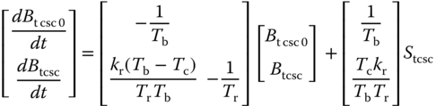
- – A cost function is defined as
- It penalizes deviations of
 from a reference trajectory
  and increments of
 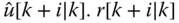 defines an ideal trajectory along which the plant returns to a set-point trajectory
  , and it can be replaced by
  in (9.2). Qi and Ri are weight matrices. Np is the number of simulations steps covered by Hp, that is to say
  . Similarly,
  . Nw means that the deviations of
  are penalized from the Nwth simulation step. During one Δt, it is assumed that
  is constant at each simulation step.
 - – The optimal sequence of
 is the one that minimizes V[k]:
9.3
is the one that minimizes V[k]:
9.3
- This is a Quadratic Programming (QP) problem, which can be solved by interior point methods, active set methods, and so on.
- – Once an optimal sequence of
 is chosen, only the first element
  is applied to the plant.
 - – The above cycle of prediction, optimization, and application is repeated at subsequent control times, in order to make
 return back to
  .
.

9.2.2 Damping Controller Models
In this section, the models of damping controllers considered in this chapter are described to facilitate readers' understanding of the developed MPC controllers. First, an IEEE Type DC1 model is adopted to represent exciter dynamics, as shown in Figure 9.2.

Figure 9.2 Exciter block diagram.
Vt is terminal voltage of the generator after load compensator; Efd is excitation voltage; Vs are supplementary inputs for the exciter, which could be PSS/MPC signals. Defining Vtr, Vas, Vr, Efd, Rf as state variables, the dynamics are described by

A PSS with the structure in Figure 9.3 is used to produce a supplementary signal Vs for the exciter.

Figure 9.3 PSS block diagram.
Its dynamics are described in the following equation, through state variables pss1, pss2, and pss3:

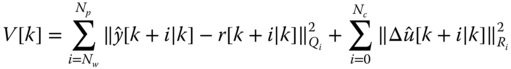
TCSC is modeled by the block diagram in Figure 9.4.

Figure 9.4 TCSC block diagram.
Its dynamics are determined by
More details about these models are given in [19].

Figure 9.5 MPC for generator.
9.3 MPC for Damping Oscillations
9.3.1 Outline of Idea
Figure 9.5 illustrates how to apply MPC to damp oscillations of one generator. Angular speed is considered as the controlled output y. A cost function penalizes deviations of ![]() from the reference speed ω0 over a prediction horizon Hp. At a control time k, MPC calculates a supplementary signal
from the reference speed ω0 over a prediction horizon Hp. At a control time k, MPC calculates a supplementary signal ![]() and combines it with PSS output Vpss as the Vs input of exciter to minimize the deviations. At subsequent control time k+i, the above process is repeated, and
and combines it with PSS output Vpss as the Vs input of exciter to minimize the deviations. At subsequent control time k+i, the above process is repeated, and ![]() is continuously updated following changes in operation conditions. In this way, the angular speed
is continuously updated following changes in operation conditions. In this way, the angular speed ![]() is forced to return back to ω0.
is forced to return back to ω0.
In a multi-generator system, the cost function is redefined to penalize deviations of all angular speeds. MPC signals are applied to each exciter to optimize and coordinate their damping effects. As well as exciters and PSSs, a TCSC on one inter-area tie line is also investigated in this chapter. As shown in Figure 9.6, the MPC signal ![]() adjusts the susceptance Btcsc, and in this way changes transmission power through the tie line to reduce oscillations.
adjusts the susceptance Btcsc, and in this way changes transmission power through the tie line to reduce oscillations.

Figure 9.6 MPC for TCSC.
9.3.2 Mathematical Formulation
The dynamics of different devices in power systems can be represented by differential equations similar to (9.4), (9.5), and (9.6). All differential equations and network algebraic equations are combined according to network topology. So, power system dynamics can be represented by the following continuous state space model:
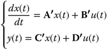
Here, A′ denotes the state matrix; B′ is the input matrix; C′ is the output matrix and D′ is the feed forward matrix. x(t) consists of all state variables; u(t) represents a vector of control inputs; y(t) is a vector of system outputs. Since there is normally no direct connection between u(t) and y(t), D′ is assumed to be zero.
Based on (9.7), the transition at an initial time t0 for a small simulation step of δ is
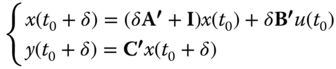
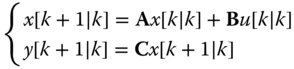
If t0 is labeled as time k, (9.8) can be rewritten as
where ![]() and
and ![]() .
.
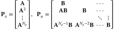
Based on current system state ![]() , future
, future ![]() over a time horizon Hp is calculated by iterating (9.9) Np times
over a time horizon Hp is calculated by iterating (9.9) Np times ![]() :
:
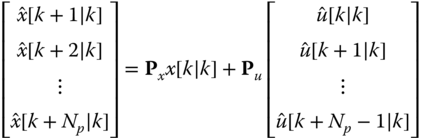
where
The corresponding ![]() is calculated by the second equation of (9.9). The MPC control objective is defined as
is calculated by the second equation of (9.9). The MPC control objective is defined as

In order to damp oscillations as soon as possible, (9.12) does not penalize ![]() increments. Equation 9.12 is subject to the following inequality constraints:
increments. Equation 9.12 is subject to the following inequality constraints:

where z denotes a vector of constrained operation variables such as bus voltage or line current.

Figure 9.7 Centralized MPC.
9.3.3 Proposed Control Schemes
9.3.3.1 Centralized MPC
A centralized MPC controller is first developed, as shown in Figure 9.7 [20]. It is assumed that a complete system model from an Energy Management System (EMS) is available, which can be refreshed from time to time following changes of load, generation, and grid topology. Every Δt seconds, the MPC controller collects current states ![]() . It then computes an open loop sequence of
. It then computes an open loop sequence of ![]() by solving (9.12). It applies the first control
by solving (9.12). It applies the first control ![]() to exciters and TCSC, and repeats the previous process at subsequent control times.
to exciters and TCSC, and repeats the previous process at subsequent control times.
9.3.3.2 Decentralized MPC
However, it is often not feasible to apply centralized control in large-scale systems due to control complexity and constraints on information exchange. Moreover, even if fully centralized control would be feasible, it is not necessarily desirable to do so due to considerations of reliability/vulnerability.
An alternative is to break down a complex control problem into manageable subproblems that are only weakly related to each other and can be independently solved. Firstly, decentralized control uses local variables and significantly reduces communication cost. Secondly, decentralized control is more reliable than centralized control, since it can tolerate a broad range of uncertainties, both within subsystems and in their interconnections. Finally, when the information exchange among subsystems is restricted, the decentralized structure becomes an essential design constraint [21]. Therefore, the above centralized MPC is further extended into a decentralized one [22]. As with any other decentralized controls, two problems are to be solved, namely decomposition and coordination.
A large-scale control problem can be decomposed into subproblems through two kinds of approaches:
- – Modeling–decomposition: construction of a global system model followed by an optimal decomposition into subsystems according to structural properties of the system and control problems under consideration [23].
- – Decomposition–modeling: a decomposition of a whole system is imposed by oscillation modes and administrative areas, and hence the modeling of subsystems has to follow the decomposition already given.
Considering restrictions on information exchange in certain power grids, it is quite difficult to construct an exact system-wide model and then decompose it. So it is preferred to consider the second approach to decompose a large power system.

Figure 9.8 Decomposition of a two-area system.
The decomposition adopted is demonstrated in a two-area system in Figure 9.8. This system is decomposed a priori into two areas, by replacing the tie line with an equivalent load and an equivalent generator. Then each area is modeled and an MPC controller is developed for it. Accordingly, the control objective of (9.12) is rewritten as the simultaneous and parallel resolution for the following area-wise optimization problem (subscript m refers to area m):

Each MPC controller solves its optimization subproblem using a detailed model of its own area and a possibly very rough model of the remaining areas (typically a black box model). It then applies the first element of the optimal control sequence to its exciters or TCSC and observes the resulting effects to proceed.
Due to the interaction among subsystems, it is necessary to coordinate area-wise MPC controllers for damping system-wide oscillations. First, MPC controllers could negotiate or exchange useful information. For example, they can inform their neighbors about what they intend to do and pass along measurements that others may not be able to sense directly [24]. In [25], Lagrange penalties on common variables between subsystems are exploited to judge the coherency of MPC computations, and any controls are not applied before Lagrange penalties converge to a pre-defined small positive constant.
However, communicating and negotiating among different areas requires considerable communications infrastructure. In today's large interconnected systems, lack of communication infrastructure is a main obstacle for implementing advanced control schemes. Upgrading this infrastructure is costly and will remain an issue at least in the near future. In addition, negotiating maybe misses good control opportunities since oscillations evolve continuously and fast. Consequently, instead of explicit communication/negotiation, an implicit coordination scheme is used in this context. Specifically, each subsystem solves its own oscillation problem, and overall system stability emerges from these area-wise controls [26], with the help of a common control objective that makes all angular speeds return to the reference speed.
9.3.3.3 Hierarchical MPC
Hierarchical control is a mixture of centralized control and decentralized control. It not only reduces the computation and communication needed by a centralized controller, but also coordinates individual decentralized controllers. In [27], a wide area central controller is responsible for decoupling subsystem dynamics and calculating the interactions among them for lower-level local controllers. Reference [28] proposes a two-loop hierarchical structure: a local loop based on a machine speed signal and a global loop based on a differential frequency between two remote areas. The total PSS signal is the sum of control components generated by these two loops.
In this section, the previous area-wise MPC is further reinforced by adding a group of device-wise MPC controllers that works on a generator in order to further improve control robustness, as shown in Figure 9.9 [29]. Compared with area-wise MPC controllers in the upper level, device-wise MPC controllers in the lower level only consider the dynamic behaviors of one generator. They calculate supplementary signals for exciters in order to make generators run at the reference speed, as described in (9.15) (subscript n refers to generator n):

Device-wise MPC controllers need less time to measure, compute, and apply their controls, so that they can update their controls more frequently following changes of system states, and thus approach their control targets in a possibly better way. In addition, when area-wise MPC controllers can't work normally, device-wise MPC controllers are designed to work independently with the aid of internal control objectives.

Figure 9.9 Hierarchical MPC.
Two ways of coupling area-wise MPC controllers and device-wise MPC controllers are investigated:
- – Input-base coupling (named hierarchical MPC I and indicated by the upper part of Figure 9.9): every Δt seconds, area-wise MPC controller m collects subsystem states and calculates
 for exciters under its authority. It sends
  to device-level MPC controllers as their decision bases. Every Δtlow seconds, the latter compute a correction
  depending on their local measurements, and combine
  with
with  as the supplementary input for the exciter.
 - – Set-point coupling (named hierarchical MPC II and indicated by the lower part of Figure 9.9): area-wise MPC controller m solves an optimization problem in (9.14) and sends the predicted
 during next Δt seconds to device-wise MPC controller n as its set-points. The latter calculates supplementary input
  in order to drive the speed of the controlled generator to reach the given set-points.
Control effects of a device-wise MPC controller depend not only on its controls, but also on states and controls of other MPC controllers existing in a same area. Therefore, these controllers are further coordinated with the help of area-wise MPC controllers. For a device-wise MPC controller, subsystem states and controls can be divided into two categories: its internal states and controls, and external states and controls related to other MPC controllers. Every Δt seconds, an area-wise MPC controller sends predicted states and controls to device-wise MPC controllers. When the latter calculate their controls, they take predicted external states and controls as simulation scenarios reflecting interactions among different controllers. The model of a device-wise MPC controller n is thus represented as follows:

where ![]() ; xn and un include the internal states and controls of MPC controllers n; An and Bn are the parts of A and B that are relative to xn; xn.ext and un.ext refer to external states and controls. The external states and controls are considered constant during one period of Δt, and hence the item “constant” is unchanged.
; xn and un include the internal states and controls of MPC controllers n; An and Bn are the parts of A and B that are relative to xn; xn.ext and un.ext refer to external states and controls. The external states and controls are considered constant during one period of Δt, and hence the item “constant” is unchanged.
9.4 Test System & Simulation Setting
The developed MPC controllers are investigated on a 16-generator, 70-bus reduced-order representation of New England and New York systems in Figure 9.10 [5]. It contains five coherent areas: areas A1–A3 respectively contain an equivalent generator representing an external equivalent system, namely generators 14, 15, and 16. Area A4 consists of generators 10–13, and Area A5 includes generators 1–9. All generators are represented by sub-transient models. They are equipped with exciters as well as Turbine Governors (TGs). PSS controllers are also installed on the generators. The loads consist of 50% constant current loads and 50% constant impedance loads. Simulations are performed on a MATLAB based software platform, Power System Toolbox (PST) [19]. The work of this chapter focuses on the inter-area oscillations between A4 and A5, which are connected to each other by the tie lines 1-2, 1-27, and 8-9. The last line is equipped with a TCSC.
x includes state variables of generators, exciters, PSSs, TGs, and TCSC. y consists of angular speeds. u is a vector of supplementary controls for exciters and TCSC, which is constrained to [-0.1 0.1]. A simulation step δ=0.005 s is used to formulate system dynamics in (9.8). Every Δt=0.1 s, the centralized MPC controller and area-wise decentralized controllers refresh their controls. The prediction horizon is set to 1.5 s (namely Hp=15) and the control horizon Hc is 3. In (9.12), (9.14), and (9.15), deviations of predicted outputs from the reference are weighted uniformly and independently, that is, all Q are identity matrices. A temporary three-phase short-circuit to ground at bus 1 (cleared by opening the tie line 1-2 followed by its reconnection after a short delay) causes poorly damped oscillations, which can be described by the temporal evolution of power flow through tie line 1-2 P1-2 and the angular speed of generator 1 Spd1 (dashed lines in Figures 9.11 and 9.12).

Figure 9.10 Test system.
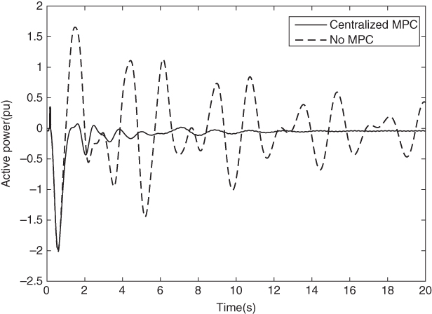
Figure 9.11 P1-2 in ideal conditions.

Figure 9.12 Spd1 in ideal conditions.
9.5 Performance Analysis of MPC Schemes
9.5.1 Centralized MPC
9.5.1.1 Basic Results in Ideal Conditions
Ideal conditions mean complete state observability and controllability, without considering SE errors and control delays. Control effects are represented by the transmission power in tie line 1-2 and the angular speed of generator 1, as shown by the solid lines in Figures 9.11 and 9.12. Compared with the system response without MPC, settling time is decreased to approximately 10 s. Figures 9.13 and 9.14 show MPC signals for the exciter on generator 1 and for the TCSC.
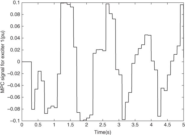
Figure 9.13 MPC signal for exciter 1.

Figure 9.14 MPC signal for TCSC.
9.5.1.2 Results Considering State Estimation Errors
At control time k, MPC uses ![]() from a state estimator and WAMS measurements as an initial value for predicting future states and outputs. Consequently,
from a state estimator and WAMS measurements as an initial value for predicting future states and outputs. Consequently, ![]() imprecision may have a detrimental effect on MPC control effects. In order to compensate for this imprecision, the difference
imprecision may have a detrimental effect on MPC control effects. In order to compensate for this imprecision, the difference ![]() between
between ![]() and its corresponding predicted value at the previous control time k-1 is added to MPC prediction:
and its corresponding predicted value at the previous control time k-1 is added to MPC prediction:

It is assumed that ![]() is refreshed at each control time, and then remains unchanged over the entire prediction horizon.
is refreshed at each control time, and then remains unchanged over the entire prediction horizon.
To simulate SE errors, ±10% uniformly distribution pseudorandom errors are superimposed on exact states. The results are shown in Figure 9.15. As expected, SE errors affect MPC performance in terms of oscillation magnitude and settling time. On the other hand, it is observed that ![]() correction considerably improves damping effects.
correction considerably improves damping effects.

Figure 9.15 Spd1 with SE errors.

Figure 9.16 Input u and delay τ.
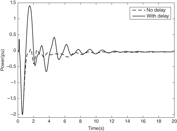
Figure 9.17 P1-2 with delay.
9.5.1.3 Consideration of Control Delays
The proposed MPC controller takes time to measure, compute, and apply its controls. Therefore, control delays are further added to MPC implementation. There are two possibilities to assess the impact of delays: apply controls as soon as they are available or after a common time interval. Here, assuming that all measurements are taken synchronously, a common delay of τ = 0.05 s is applied to all controllers. As shown in Figure 9.16, at a control time k, the MPC controller computes ![]() . However because of
. However because of ![]() can't be applied immediately, but from
can't be applied immediately, but from ![]() . Between kΔt and
. Between kΔt and ![]() ,
, ![]() (which is calculated at time k-1) is implemented. The system response under this treatment is shown in Figure 9.17. It is clear that the response taking into account delays is worse than the one only considering SE corrections, but still quite superior to the response without MPC.
(which is calculated at time k-1) is implemented. The system response under this treatment is shown in Figure 9.17. It is clear that the response taking into account delays is worse than the one only considering SE corrections, but still quite superior to the response without MPC.
9.5.2 Distributed MPC
The test system is re-divided into two parts: part 1 consists of A1-A4 and part 2 is the rest. TCSC is assigned to part 1 as its control resource. One area-wise MPC controller is installed in two parts. MPC1 calculates ![]() for exciters 10-16 and TCSC; MPC 2 is responsible for exciters 1-9. System response is shown in Figure 9.18.
for exciters 10-16 and TCSC; MPC 2 is responsible for exciters 1-9. System response is shown in Figure 9.18.
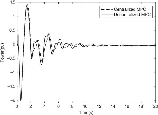
Figure 9.18 P1-2 with decentralized MPC.
It is observed that the distributed MPC yields similar control effects to the centralized MPC. This is due to the chosen decomposition method. The system is decoupled by replacing the exchange power with one load and one generator whose values are equal to the exchange power at steady state. Hence, the subsystem models obtained in this way contain the information about this power. In addition to the explicit control objective of (9.14), the area-wise MPC controllers have another implicit objective, namely restoring the exchange power to its steady state value. This actually further strengthens the coordination between the two area-wise MPC controllers.
9.5.3 Hierarchical MPC
Device-wise MPC controllers are installed on each generator. The area-wise MPC controllers use the same simulation parameters as the distributed MPC. The device-wise MPC controllers refresh their controls every Δtlow = 0.01 s and use a control horizon Hcl = 5. The prediction horizon Hpl is set to 60 in part 1 and 40 in part 2. Figure 9.19 shows that compared with the distributed MPC, the hierarchical one further slightly improves control effects.

Figure 9.19 P1-2 with hierarchical MPC1.
As explained in the Section 9.3.3.3, the advantage of hierarchical MPC is to further improve control robustness. So, next, the robustness of hierarchical MPC is verified through the following examples:
- – increasing Δt of area-wise controllers from 0.1 s to 0.2 s;
- – losing area-wise MPC controller in part 1 during the first 5 s after the disturbance;
- – incomplete measurements—it is assumed that only states of generators 10-12 and generators 1-4 are available for area-wise MPC controllers;
- – communication failure between area-wise MPC controllers and device-wise MPC controllers—it is assumed that MPC controllers on generators 5-9 and 12-14 can't receive signals from area-wise MPC controllers.
The left part of Figure 9.20 compares two methods of coupling for hierarchical MPC. Utilizing set-point coupling, device-wise MPC controllers take worse predicted values with larger errors as their set-points because MPC prediction precision deteriorates with increasing Δt. However, in input-base coupling, although area-wise MPC prediction becomes worse, device-wise MPC controllers can continuously correct input bases utilizing local measurements and control objectives. Therefore, the latter yields better control effects. So in other test cases, input-base coupling is used—namely hierarchical MPC I.

Figure 9.20 Spd1 with Δt of 0.2 seconds.
Figures 9.20–9.23 give the response of transmission power P1-2 for each test case. It is shown that the hierarchical MPC is more robust than the distributed one because of its better performances in different test cases.


Figure 9.23 P1-2 with communication failure.
9.6 Conclusions and Discussions
In contrast to traditional damping control methods that focus on oscillation modes and damping ratios, this chapter interprets damping control as a dynamic process control problem over a future time horizon. This problem penalizes future deviations of generator speeds from the reference speed, and solving it produces supplementary inputs for existing damping controllers. These inputs are refreshed at each control time, which is actually equal to adaptively adjust damping controllers' parameters following changes in operation condition, in order to improve and coordinate their damping effects.
MPC is a good solution for dynamic process control. Therefore, this chapter attempts to apply it to produce supplementary inputs for existing damping controllers. First, a centralized MPC is developed to demonstrate this idea. Next, it is extended into a decentralized MPC for viability in large power systems. Finally, a hierarchical MPC scheme is proposed with the aim of enhancing control robustness. The performances of the three MPC schemes are tested on a 70-bus system. It is observed that the distributed scheme appears to be a feasible control strategy for large systems while the hierarchical MPC further improves control effects, and at the same time offers better robustness.
There are still many improvements to be made for the proposed MPC schemes before they can be applied in real power systems. First, an exact model is a prerequisite for MPC to produce good damping effects. But even in a subsystem, it is not easy to build a complete and exact model. And such a model involves considerable communication when MPC is active. So an alternative is to build reduced-order models that can describe oscillation dynamics and need fewer measurements. The area-wise controllers in the decentralized MPC are coordinated in an implicit way, through a common control objective for subsystems. This coordination should be further verified in multi-area systems. Finally, in the hierarchical MPC, corrections from device-wise MPC controllers can be considered as disturbances for area-wise MPC controllers. In this chapter, the limits of corrections are determined through repeated simulation trials. Further work needs to be done on coordinating the two kinds of MPC controllers.
References
- 1 E. Grebe, J. Kabouris, S. Lopez Barba, W. Sattinger, et al, “Low Frequency Oscillations in the Interconnected System of Continental Europe”, Proceedings of the IEEE Power and Energy Society General Meeting 2010, July 25–29, 2010, Minneapolis, MN, United States.
- 2 P. Korba and K. Uhlen, “Wide-area Monitoring of Electromechanical Oscillations in the Nordic Power System: Practical Experience”, IET Generation, Transmission, Distribution, Vol. 4, No. 10, May 2010, pp. 1116–1126.
- 3 Y. Liu, J. R. Gracia, T. J. King and Y. L. Liu, “Frequency Regulation and Oscillation Damping Contributions of Variable-Speed Wind Generators in the U.S. Eastern Interconnections (EI)”, IEEE Transactions on Sustainable Energy, Vol. 6, No. 3, July 2015, pp. 951–958.
- 4 D. N. Kosterev, C. W. Taylor and W. A. Mittelstadt, “Model Validation for the August10, 1996 WSCC System Outage”, IEEE Transactions on Power Systems, Vol. 14, No. 3, Aug. 1999, pp. 967–979.
- 5 G. Rogers, Power System Oscillations. Norwell, Massachusets, USA: Kluwer Academic Publishers, 2000.
- 6 R. Preece, J. V. Milanović, A. M. Almutairi and O. Marjanovic, “Damping of Inter-area Oscillations in Mixed AC/DC Networks using WAMS based Supplementary Controller”, IEEE Transactions on Power Systems, Vol. 28, No. 2, May 2013, pp. 1160–1169.
- 7 R. Majumder, B. Chaudhuri and B. C. Pal, “A Probabilistic Approach to Model-based Adaptive Control Damping of Interarea Oscillations in Power Systems”, IEEE Transactions on Power Systems, Vol. 20, No. 1, Feb. 2005, pp. 367–374.
- 8 S. J. Qin and T. A. Badgwell, “A Survey of Industrial Model Predictive Control Technology”, Control Engineering Practice, Vol. 11, No. 7, July 2003, pp. 733–764.
- 9 R. Scattolini, “Architectures for Distributed and Hierarchical Model Predictive Control - A Review”, Journal of Process Control, Vol. 19, No. 5, May 2009, pp. 723-731.
- 10 F. Capitanescu and L. Wehenkel, “A New Iterative Approach to the Corrective Security-Constrained Optimal Power Flow Problem”, IEEE Transactions on Power Systems, Vol. 23, No. 4, Nov. 2008, pp. 1533–1541.
- 11 B. Otomega, A. Marinakis, M. Glavic and T. V. Cutsem, “Model Predictive Control to Alleviate Thermal Over Loads”, IEEE Transactions on Power Systems, Vol. 22, No. 3, Aug. 2007, pp. 1384–1385.
- 12 J. J. Ford, G. Ledwich and Z. Y. Dong, “Efficient and Robust Model Predictive Control for First Swing Transient Stability of Power Systems using Flexible AC Transmission Systems Devices”, IET Generation, Transmission, Distribution, Vol. 2, No. 5, Sept. 2008, pp. 731–742.
- 13 T. A. Short, D. A. Pierre and J. R. Smith, “Self-tuning Generalized Predictive Control for Switched Capacitor Damping of Power System Oscillations”, Proceedings of the 28th conference on decision and control, Dec. 1989, Florida, USA.
- 14 N. P. Johansson, H. P. Nee and L. Angquist, “An Adaptive Model Predictive Approach to Power Oscillation Damping Utilizing Variable Series Reactance FACTS Devices”, Proceedings of the 41st International Universities Power Engineering Conference, Sept. 2006, Newcastle, UK.
- 15 L. Wang, H. Cheung, A. Hamlyn and R. Cheung, “Model Prediction Adaptive Control of Inter-area Oscillations in Multi-generators Power Systems”, Proceedings of IEEE Power and Energy Society General Meeting, July 2009, Calgary, Canada.
- 16 R. Majumder, B. Chaudhuri and B. C. Pal, “A Probabilistic Approach to Model-based Adaptive Control for Damping of Interarea Oscillations”, IEEE Transactions on Power Systems, Vol. 20, No. 1, Feb. 2005, pp. 367–374.
- 17 B. Chaudhuri, R. Majumder and B. C. Pal, “Application of Multiple-model Adaptive Control Strategy for Robust Damping of Interarea Oscillations in Power System”, IEEE Transactions on Control Systems Technology, Vol. 12, No. 5, Sept. 2004, pp. 727–736.
- 18 J. Maciejowski, Predictive Control with Constraints, Prentice Hall, Harlow, England, 2002.
- 19 J. Chow, and G. Rogers, “Power System Toolbox Version 3.0”, http://www.eps.ee.kth.se/personal/vanfretti/pst/Power_System_Toolbox_Webpage/PST.html, 2016.
- 20 D. Wang, M. Glavic and L. Wehenkel, “A New MPC Scheme for Damping Wide-Area Electromechanical Oscillations in Power Systems”, Proceedings of IEEE Power and Energy Society PowerTech, June 2011, Trondheim, Norway.
- 21 D. D. Siljak and A. I. Zecevic, “Control of Large-Scale Systems: Beyond Decentralized Feedback”, IEEE Transactions on Power Systems, Vol. 20, No. 1, Feb. 2005, pp. 367–374.
- 22 D. Wang, M. Glavic and L. Wehenkel. “Distributed MPC of Wide-Area Electromechanical Oscillations of Large-scale Power Systems”, Proceedings of the 16th intelligent system applications to power systems (ISAP), Sep. 2011, Crete, Greece.
- 23 N. Motee and B. Sayyar-Rodsari, “Optimal Partitioning in Distributed Model Predictive Control”, Proceedings of the 2003 American control conference, June 2003, Colorado. USA.
- 24 S. Talukdar, D. Jia, P. Hines and B. H. Krogh, “Distributed Model Predictive Control for the Mitigation of Cascading Failures”, Proceedings of the 44th IEEE conference on decision and control, Dec. 2005, Seville, Spain.
- 25 R. R. Negenborn and B. S. Rodsai, “Multi-agent Model Predictive Control with Applications to Power Networks”, PhD thesis, Delft university of Technology, 2007.
- 26 A. N. Venkat, I. A. Hiskens, J. B. Rawlings and S. J. Wright, “Distributed MPC Strategies with Application to Power System Automatic Generation Control”, IEEE Transactions on Control Systems Technology, Vol. 16, No. 6, Nov. 2008, pp. 1192–1206.
- 27 I. Kamwa, R. Grondin and Y. Hebert, “Wide-area Measurement based Stabilizing Control of Large Power Systems - A Decentralized/Hierarchical Approach”, IEEE Transactions on Power Systems, Vol. 16, No. 6, Feb. 2001, pp. 136–153.
- 28 F. Okou, L. A. Dessaint and O. Akhrif, “Power Systems Stability Enhancement Using a Wide-area Signals based Hierarchical Controller”, IEEE Transactions on Power Systems, Vol. 20, No. 3, Aug. 2005, pp. 1465–1477.
- 29 D. Wang, M. Glavic and L. Wehenkel, “Considerations of Model Predictive Control for Electromechanical Oscillations Damping in Large-scale Power Systems”, International Journal of Electric Power and Energy Systems, Vol. 58, 2014, pp. 32–41.