
Chapter 6
Performance Indicator-Based Real-Time Vulnerability Assessment
Jaime C. Cepeda1, José Luis Rueda-Torres2, Delia G. Colomé3 and István Erlich4
1Head of Research and Development, and University Professor Technical Development Department, and Electrical Energy Department Operador Nacional de Electricidad CENACE, and Escuela Politécnica Nacional EPN, Quito, Ecuador
2Assistant professor of Intelligent Electrical Power Systems, Department of Electrical Sustainable Energy, Delft University of Technology, The Netherlands
3Professor of Electrical Power Systems and Control, Institute of Electrical Energy, Universidad Nacional de San Juan, Argentina
4Chair Professor of Department of Electrical Engineering and Information Technologies, Head of the Institute of Electrical Power Systems, University Duisburg-Essen, Duisburg, Germany
6.1 Introduction
Electric power systems usually support perturbations which, depending on their severity, eventually could initiate cascading events that might cause total or partial blackouts [1]. In this context, vulnerability assessment needs to be done in order to determine the necessity of triggering different types of protection mechanisms (i.e., System Integrity Protection Schemes (SIPS) or Special Protection Schemes (SPS)) designed to attenuate the risk of these possible blackouts [2, 3]. However, the conditions that lead a system to blackouts are not easy to identify because the process of system collapse depends on multiple interactions [4]. Therefore, vulnerability assessment should be done considering these interactions that, in fact, relate several electrical phenomena that can be defined as vulnerability symptoms [5].
Vulnerability assessment is carried out by checking the system performance under the severest contingencies with the purpose of detecting the conditions that could initiate cascading failures and might provoke system collapses [6]. A vulnerable system can be defined as a system that operates with a “reduced level of security that renders it vulnerable to the cumulative effects of a series of moderate disturbances” [6]. The concept of vulnerability involves the system security level (static and dynamic security) [7] and the tendency to change its conditions into a critical state, known as the “Verge of Collapse State” [5]. A Vulnerable Area is a specific section of the system where vulnerability begins to develop. The occurrence of an abnormal contingency in the vulnerable areas and highly stressed operating conditions define a system in the Verge of Collapse State. Vulnerable areas are characterized by, in total, five different symptoms of system stress: transient stability, poorly-damped power oscillations, voltage instability, frequency deviations outside limits, and overloads, as analyzed in Chapter 1.
Many methods have been proposed for vulnerability assessment [4, 6]. Conventional methods are based on steady state or dynamic simulations of contingencies, that is, static security assessment (SSA) or dynamic security assessment (DSA) [4, 6–9], which can also be associated to a specific probability of occurrence [4, 6]. These methods require long processing times, which restricts online applications. Modern high-performance computing (HPC) techniques have improved calculation times, permitting online applications [8], but does not allow real-time uses. Emerging technologies such as Phasor Measurement Units (PMUs) and Wide Area Monitoring Systems (WAMS), which provide voltage and current phasor measurements with updating periods of one cycle, have allowed the development of modern approaches for real-time dynamic vulnerability assessment (DVA) [9–11]. Other emerging methods permit identification of indicators or patterns that show system vulnerability, which use artificial intelligence [6] or modern data mining tools [10, 11]. Some of these approaches permit assessment of the post-contingency system security level, but they do not consider the fact that vulnerability begins to develop in specific areas of the system, which instead is tackled in [12] using some performance indicators. Moreover, most of these approaches have been focused on analyzing only one symptom of vulnerability, while the approach that considers several phenomena only allows prediction of power system post-contingency dynamic vulnerability status [11] but does not consider the valuation of the security level via performance indicators.
This chapter presents a comprehensive real-time vulnerability assessment methodology oriented to determine vulnerable areas of an electric power system and to assess vulnerability of each one of them, considering both aspects involved in the vulnerability concept, that is: (i) assessment of the system's tendency to reach a critical state, and (ii) evaluation of the actual security level. In the present chapter, the methodology for identifying vulnerable areas in real time, based on electrical coherency, is firstly introduced. Then, the evaluation of system security level due to the three short-term stability phenomena (i.e., transient, voltage, and frequency stability (TVFS)) is presented. After this, the assessment for oscillatory stability and overloads, that is, the slowest phenomena, is defined. Finally, both tasks involved in the concept of vulnerability are joined and the complete vulnerability assessment is presented. All of these vulnerability symptoms are evaluated via different key performance indicators (KPIs) that also combine the results of the post-contingency vulnerability status prediction based on Dynamic Vulnerability Regions (DVR) presented in Chapter 5 by using arrays of logic gates.
6.2 Overview of the Proposed Vulnerability Assessment Methodology
The present chapter presents a comprehensive methodology to assess post-contingency system dynamic vulnerability in real time by using PMU measures as input data. This premise is based on the fact that after a contingency occurs, power system variables (i.e., voltage phasors, current phasors, and frequencies) begin to change, and these variables can be measured, in real time, by PMUs adequately located throughout the system. Using these data as inputs, the proposed real-time DVA methodology is capable of giving early warning alerts about possible system blackouts. The framework of the proposal is schematically sketched in Figure 6.1. As can be seen, the results of the complete assessment are several KPIs that evaluate the power system vulnerability condition.

Figure 6.1 Framework of the proposed real-time assessment methodology.
The procedure depicted in Figure 6.1 describes the steps to be followed in real time to achieve the proposed post-contingency vulnerability assessment (VA). The scheme begins with the PMU data acquisition at each updating period. These data are then received and pre-processed in the control center in order to filter possible noise and debug potential outliers (this chapter assumes that this pre-processing step has already been accomplished).
The approach allows carrying out VA through identifying vulnerable areas and ranking them according to their grade of vulnerability, which is evaluated via several KPIs, taking into account several signals of system stress that have been split into “faster” and “slower” phenomena depending on their evolution timeframe. For this purpose, both tasks involved in the vulnerability concept are assessed through the prediction of the future vulnerability status and the evaluation of the actual state security level. Afterwards, several performance indices are computed that can be seen as a measure of the post-contingency system vulnerability per each area.
In real time, the power system is firstly partitioned into coherent electric areas via an adequate mathematical tool that analyzes coherency from the PMU dynamic data. Then, five vulnerability indices (indicators) that reflect the performance of the system as regards the symptoms of system vulnerability are computed for each electric area. These indicators cover the assessment of both tasks involved in the vulnerability concept.
6.3 Real-Time Area Coherency Identification
As noted in [13], interconnected power systems are usually partitioned into areas for different reasons such as reduction of required measurements for each coherent area, improvement of corrective control actions, or facilitation of system modeling in the case of huge or complex interconnected systems. The objective of system partitioning in this chapter is to detect, in real time, the vulnerable areas in which the possibility of a cascading event beginning exists.
The bus where a PMU is located represents the “centroid” of a coherent electrical area [14], which can be seen as the “associated PMU coherent area.” Since the coherent electrical areas can change depending on the operating state and the actual contingency, it is necessary to analyze the possibility of existing coherency between the associated PMU coherent areas. Then, the aim of the real-time area coherency identification is to join two or more associated PMU coherent areas into “zones,” if coherency between them is detected.
Hence, the recursive clustering approach for decomposing large power systems into coherent electrical areas presented in [14], and initially introduced in [13], is used. This coherency calculation method is adapted to be used in real time. In this connection, the three dissimilarity matrices for voltage angle, voltage magnitude, and frequency (Dθ, DV, and DF) [14] are built using the data measured by the PMUs located in the power system. Then, the size of these matrices is (NPMU × NPMU), with NPMU being the number of PMUs placed in the system.
Since this clustering algorithm is an iterative method, it improves its results according to the number of data items used to find the clusters, which are actualized when each phasor measurement arrives to the control center. Because of this fact, the implemented algorithm will be run at each PMU updating period, and the coherent groups might change during the event evolution.

Once the power system is partitioned into real-time coherent electrical areas, several performance indicators associated with each vulnerability symptom are calculated for each electrical area, as explained in the next sections.
One important aspect to be considered before applying the suggested algorithm is to specify the boundaries of the associated PMU coherent areas a priori, which will be discussed in the following subsection.
6.3.1 Associated PMU Coherent Areas
Since fast coherency may change depending on the operating state and the contingency magnitude, the number and the structure of the coherent electrical areas might be different. Monte Carlo (MC)-based dynamic simulations and clustering analysis, similar to those applied for placing the PMUs in [14], can be carried out in order to analyze the different possibilities of coherent areas for different operating states and contingencies. In this connection, once PMUs are placed (via the method depicted in [14]), a probabilistic analysis of coherent areas has to be done in order to determine the most representative group of coherent buses associated to each PMU (i.e., the probabilistic areas associated to PMUs), which will permit structuring a database for real-time use.

Figure 6.2 39-bus-system associated PMU areas: (a) associated PMU 1 area, (b) associated PMU 2 area, (c) associated PMU 3 area, (d) associated PMU 4 area, (e) associated PMU 5 area, (f) associated PMU 6 area.
Thus, a probabilistic analysis of the results of the fast dynamic coherency Monte Carlo analysis described in [14], via histograms, would reveal those buses belonging to each associated PMU area that present the highest frequency. The real-time area coherency identification is then used to join these associated PMU areas if there is high coherency behavior during the development of the actual contingency.
For illustrative purposes, the identification of the probabilistic areas associated to PMUs, based on MC-based simulations is carried out to the IEEE New England 39-bus, 60 Hz and 345 kV test system, previously presented in Figure 5.4 of Chapter 5, including the PMUs already located [14]. Figure 6.2 presents histograms of the 39-bus-system probabilistic coherency area results, showing the buses that belong to the same area as each PMU already located (i.e., areas associated to each PMU). From the histograms, the buses that present the highest frequencies are selected to compose each associated PMU coherent area, considering that each PMU can belong to only one area as the basic premise. Table 6.1 shows the 39-bus-system associated PMU area resulted database.
The results are also illustrated in Figure 6.3, which present the buses that belong to each associated PMU area over the system single-line diagram. The different coherency distribution in each MC iteration is reflected in the overlap that exists between coherent areas, which can be seen in the figure.
Table 6.1 39-bus-system associated PMU area database
| PMU | Associated PMU coherent Areas/Buses |
| PMU 1 | Area 1 = {1, 2, 3, 4, 18, 25, 30, 37} |
| PMU 2 | Area 2 = {1, 6, 7, 8, 9, 31, 39} |
| PMU 3 | Area 3 = {3, 4, 5, 6, 7, 8, 10, 11, 12, 13, 14, 31, 32} |
| PMU 4 | Area 4 = {3, 15, 16, 17, 18, 19, 20, 24, 27, 33, 34} |
| PMU 5 | Area 5 = {15, 16, 19, 20, 21, 22, 23, 24, 33, 34, 35, 36} |
| PMU 6 | Area 6 = {25, 26, 27, 28, 29, 37, 38} |

Figure 6.3 39-bus-system probabilistic associated PMU areas.
6.4 TVFS Vulnerability Performance Indicators
The evaluation of each of the symptoms of a stressed system mentioned above has to be done in order to properly assess vulnerability. In this section, three vulnerability indices, which resemble the system security level as regards transient stability, short-term voltage stability, and short-term frequency stability issues (TVFS), are presented.
These indices are then joined with the results obtained from the TVFS vulnerability status prediction depicted in Chapter 5 in order to perform both tasks involved in the vulnerability concept (i.e., actual security assessment and prediction of future vulnerability status).
For illustrative purposes, dynamic simulations consisting in several contingencies where the causes of vulnerability could be transient instability, short-term voltage instability, or short-term frequency instability (TVFS) have been carried out on the 39 bus test system. These contingencies are generated by applying the Monte Carlo method. Two types of events are considered: three phase short circuits and generation outage. The short circuits are applied at different locations of the transmission lines, depending on the Monte Carlo simulation. The disturbances are applied at 0.12 s, followed by the opening of the corresponding transmission line at 0.2 s (i.e., fault clearing time tcl). Likewise, the generation to be tripped is also chosen by the Monte Carlo method, and this type of contingency is applied at 0.2 s.
Several operating states have been considered by varying the load of the PQ buses, depending on three different daily load curves. Then, optimal power flow (OPF) is performed in order to establish each operating state, using the MATPOWER package. After that, time domain simulations have been performed using the DIgSILENT PowerFactory software, so that the post-contingency PMU dynamic data could be obtained.
For instance, post-contingency dynamic responses of four different MC iterations are presented in Figures 6.4–6.7. These figures depict the simulation results of one non-vulnerable case, one transient unstable case, one voltage unstable case, and one frequency unstable case, respectively. It is possible to observe in the figures the particular dynamic signal behavior for each one of the cases, which exposes the existence of certain patterns revealing the actual system security level, as well as the future system-vulnerability-status tendency. These cases will be used as illustrative examples throughout this chapter.

Figure 6.4 39-bus-system non-vulnerable case.

Figure 6.5 39-bus-system transient unstable case.

Figure 6.6 39-bus-system voltage unstable case.

Figure 6.7 39-bus-system frequency unstable case.
6.4.1 Transient Stability Index (TSI)
The real-time transient stability index (TSI) presented in [10] can be used as a KPI for transient stability. This index is determined via the prediction of area-based center-of-inertia-(COI)-referred rotor angles using PMU measurements as input data, and is capable of giving a quick quantification of the actual TS level. The method uses an intelligent COI-referred rotor angle regressor based on Monte Carlo simulation, a support vector regressor (SVR), and PMU data as input. This regressor is used for obtaining the COI-referred rotor angles directly from PMU measurement in real time.
For real-time implementation, the previously off-line trained SVR [10] will be in charge of estimating the COI-referred rotor angles for each area associated to the PMUs, using the actual post-contingency PMU voltage phasors as inputs. Once the associated PMU COI-referred rotor angles are estimated, the recursive clustering approach for determining coherent electrical areas is first applied to these angles in order to determine the boundaries of the real-time coherent areas, as explained in Section 6.3. After the definition of real-time areas, new area-COI-referred rotor angles will be computed, representing the real-time coherency. The expressions that permit computation of these new COI-referred rotor angles are presented by (6.2) and (6.3):


where ![]() is the estimated COI-referred rotor angle of the associated PMU j-th area, v is the number of associated PMU areas that belong to the real-time area k determined by the real-time recursive coherency method, and Mj is the total inertia moment of the j-th associated PMU area, whereas MkT and
is the estimated COI-referred rotor angle of the associated PMU j-th area, v is the number of associated PMU areas that belong to the real-time area k determined by the real-time recursive coherency method, and Mj is the total inertia moment of the j-th associated PMU area, whereas MkT and ![]() denote total inertia moment and the new COI-referred-rotor angle of the k-th real-time coherent area.
denote total inertia moment and the new COI-referred-rotor angle of the k-th real-time coherent area.
Finally, using the ![]() computed value and the TSA criterion presented in [10], it is possible to establish a TSI in the range of [0, 1] for each k-th area as shown by (6.4). This TSIk will be computed after each set of PMU data arrives to the control center and might be used as an indicator of the area being imminently out-of-step:
computed value and the TSA criterion presented in [10], it is possible to establish a TSI in the range of [0, 1] for each k-th area as shown by (6.4). This TSIk will be computed after each set of PMU data arrives to the control center and might be used as an indicator of the area being imminently out-of-step:

where TSIk, and ![]() are the TS index and COI-referred rotor angle in radians of the k-th real-time area. Since TSI is conceived to give early warning, it is not necessary to compute it when COI-referred rotor angles are within a normal operating range. Then, the maximum admissible steady state COI-referred rotor angle (i.e., the maximum allowed angle determined by steady state constraints—δlim) is used as the lower limit of the TSI function.
are the TS index and COI-referred rotor angle in radians of the k-th real-time area. Since TSI is conceived to give early warning, it is not necessary to compute it when COI-referred rotor angles are within a normal operating range. Then, the maximum admissible steady state COI-referred rotor angle (i.e., the maximum allowed angle determined by steady state constraints—δlim) is used as the lower limit of the TSI function.
As an illustration, the COI-referred rotor angles for the unstable case presented in Figure 6.5 are estimated [10]. Figure 6.8 shows a comparison between the computed (solid lines) and the estimated (dotted lines) associated PMU COI-referred rotor angles for this case.

Figure 6.8 Associated PMU COI-referred rotor angles for transient unstable case of Figure 6.5.
6.4.2 Voltage Deviation Index (VDI)
In the context of vulnerability, it is a fact that bus voltages are good indicators of the health of the system. So, a voltage deviation index (VDI) can be used in order to assess vulnerability. This index has to be calculated when each phasor measurement arrives at the control center.
Since the defined vulnerability assessment timeframe covers only the short-term voltage stability phenomena, the proposed index is intended to reflect the power system voltage performance as regards the voltage dynamic period.
During this dynamic period, the under and over-voltage relays (VR) might operate when specific vulnerable conditions are reached. In this connection, the defined VDI resembles the operating characteristics of this type of relay, which is triggered when the voltage drops below a threshold value Vlower (or exceeds a threshold value Vupper) during more than a pre-defined period of time (tvmax). Figure 6.9 schematizes the definition of an under-voltage VR triggering operation.

Figure 6.9 Voltage relay triggering characteristic.
Using the previously defined VR characteristics, it is possible to define a VDI for each bus where PMUs are located, as follows:

where V is the instant i-th PMU voltage, Vlower and Vupper are the voltage threshold values, tvmax is the maximum pre-defined period of time before the VR triggers, and tn is the period of time in which ![]() or
or ![]() .
.
Then, the VDI for each real-time electric area k is determined by the following expression:
6.4.3 Frequency Deviation Index (FDI)
The frequency deviation from its rated value is a clear indicator of the dynamic effect produced by the contingency. As noted in [8], the higher the frequency deviation, the bigger the effect produced by the contingency.
Using this concept, an approach for assessing vulnerability in each area is used based on the fact that frequency can also be measured in PMUs, and these data might be used in control centers with similar updating periods and phasors.
In order to assess the effect of the frequency behavior, the frequency measured in each PMU is assessed, since the frequency is not the same in all system buses during dynamic conditions.
Typical frequency threshold value settings are 57–58.5 Hz for a 60 Hz system and 48–48.5 Hz for a 50 Hz system (Δfmax from 2.5% to 5%) [15]. Similarly, over frequency protection of generators usually has a threshold value of 61.7 Hz (Δfmax around 2.8% for a 60 Hz system) [16].
Using this information, a Frequency Deviation Index (FDI) for each PMU can be calculated as follows:

where ![]() is the frequency variation measured in PMU i, and Δfmax is the maximum admissible system frequency deviation. Notice that Δfmax changes depending on the frequency phenomenon. That is, if
is the frequency variation measured in PMU i, and Δfmax is the maximum admissible system frequency deviation. Notice that Δfmax changes depending on the frequency phenomenon. That is, if ![]() , this corresponds to an under frequency limit; otherwise, if
, this corresponds to an under frequency limit; otherwise, if ![]() corresponds to an over frequency limit.
corresponds to an over frequency limit.
Then, using the previous index per PMU, the FDI for each real-time electrical area k is determined as follows:

Figure 6.10 TSI for transient unstable case of Figure 6.5.

Figure 6.11 VDI for voltage vulnerable case of Figure 6.6.
6.4.4 Assessment of TVFS Security Level for the Illustrative Examples
In this section, the computation of each TVFS performance indicators is illustrated in order to show the real-time application of the stage involved with the evaluation of the system security level. For instance, the TSI, VDI, and FDI are computed for each one of the unstable cases presented in Figures 6.5, 6.6, and 6.7, respectively. First, the real-time coherency analysis is performed in order to partition the system into specific coherent zones (by clustering the associated PMU electric areas).
The TVFS indices per zone for each one of these unstable cases are presented in Figure 6.10 (Zone A = {Area 1, Area 4, Area 6}, Zone B = {Area 2, Area 3}, and Zone C = {Area 5}), Figure 6.11 (Zone A = {Area 1, Area 2, Area 3, Area 6}, Zone B = {Area 4}, Zone C = {Area 5}), and Figure 6.12 (Zone A = {Area 1, Area 2, Area 3, Area 6}, Zone B = {Area 4}, Zone C = {Area 5}).

Figure 6.12 FDI for frequency vulnerable case of Figure 6.7.
Note in the figures how each indicator reaches the value of “1” at 0.72 s, 3.5 s, and 15 s, respectively. At this moment, the assessment of TVFS security level gives an alert of the system collapse. Nevertheless, at the instant in which the alert is given, the system is already collapsing. Thus, the need for an early warning cannot be achieved simply by the evaluation of the actual security level by means of performance indicators. In this connection, the use of a prediction mechanism is essential in order to be able to apply any corrective action before the system collapses, which will be incorporated by the inclusion of the vulnerability status prediction results, presented in Chapter 5. This aspect will be analyzed in the next subsection.
6.4.5 Complete TVFS Real-Time Vulnerability Assessment
In this subsection, the previously defined TVFS indices (i.e., TSI, VDI, and FDI) are combined with the results obtained from the TVFS vulnerability status prediction depicted in Chapter 5 with the aim of performing both tasks involved in the vulnerability concept, that is: assessment of the actual security level, and of the system's tendency to reach a critical state.
For this purpose, a “penalty” is included into the indices depending on the result obtained from the vulnerability status prediction, taking into account the time window where the vulnerability status has been predicted and adequate arrays of logic gates. This penalty has the aim of forcing the corresponding TVFS index to the value of “1” when the vulnerability status pattern recognition results in an alert about the system's tendency to change its conditions to a critical state (i.e., when the vulnerability status prediction is set to “1”). In order to increase security, this penalty is applied only if the corresponding TVFS index has exceeded a minimum pre-specified value.
In order to determine the time windows where two or more different phenomena might occur, the statistical results of the relay tripping times and the pre-defined time windows (TWs) are used (according to explanation given in Chapter 5).
From the analysis for the 39 bus test system (see Chapter 5), TW1 and TW2 allow predicting the transient unstable cases; TW3 includes the information of voltage vulnerable cases; while TW4 and TW5 contain the patterns belonging to vulnerability caused by voltage or frequency phenomena. This analysis is summarized in Figure 6.13, whereas the corresponding defined logic schemes are presented in Figure 6.14.

Figure 6.13 Time window analysis for structuring the 39-bus-system logic schemes.

Figure 6.14 39-bus-test system logic schemes: a) TW1 ∨ TW2, b) TW3, c) TW4 ∨ TW5.
After specifying the logic schemes, the TVFS performance indicators are again computed.
The behavior of the TVFS indices for the transient unstable case is presented in Figure 6.15. Note how the real-time coherency identification method joins the pre-specified associated PMU coherent areas into a new set of coherent zones, which change during event evolution. At the beginning, four different zones are determined; but after seven samples (at around 0.34 s), the iterative algorithm improves the results, suggesting the formation of three coherent zones, which present the best final coherency distribution. Then, for this specific case, the system is partitioned into three coherent zones at the moment of vulnerability detection, that is: Zone A = {Area 1, Area 4, Area 6}, Zone B = {Area 2, Area 3}, and Zone C = {Area 5}. Figure 6.15 (a) shows how the TSI of Area C reaches the value of “1” at 0.5 s after the corresponding application of the penalty when the vulnerability status is set to “1” by the TW1 status prediction classifier. In the figure, the slope change at around 0.48 s is a product of this penalty application. Since in this case the loss of synchronism occurs at 0.9854 s (tripping of out-of-step relay OSR), the operator will have around 480 ms to perform any corrective control action.

Figure 6.15 TVFS indices for transient unstable case of Figure 6.5.
Likewise, Figure 6.16 shows the TVFS vulnerability indicators corresponding to the voltage vulnerable case presented in Figure 6.6. In this case, the real-time area coherency iterative algorithm orients the formation of three or four different coherent zones at the beginning, from which the final coherency distribution corresponds to four coherent zones. These zones are: Zone A = {Area 1}, Zone B = {Area 2}, Zone C = {Area 3}, and Zone D = {Area 4, Area 5, Area 6}.

Figure 6.16 TVFS indices for voltage vulnerable case of Figure 6.6.
The VDI of Zone C reaches the value of 1 at 2.9 s, when the vulnerability status prediction corresponding to TW3 warns about the voltage vulnerability risk. Considering that the voltage relay VR tripped at 3.42 s, the methodology allows alerting about the vulnerability risk 520 ms before it occurs.
Figure 6.17, in contrast, presents the TVFS vulnerability indices corresponding to the frequency vulnerable case of Figure 6.7. At this instant, the real-time area coherency identification detects the formation of three different coherent zones from the beginning. These zones are: Zone A = {Area 1, Area 2, Area 3, Area 6}, Zone B = {Area 4}, and Zone C = {Area 5}. The FDI of Zone A reaches the value of 1 at 9.2 s, when the vulnerability status prediction corresponding to TW5 alerts about the frequency vulnerability risk. In this case, the TVFS vulnerability assessment warns about vulnerability 3.71 s before it occurs due to the corresponding frequency relay (FR) tripping at 12.912 s.

Figure 6.17 TVFS indices for frequency vulnerable case of Figure 6.7.
6.5 Slower Phenomena Vulnerability Performance Indicators
Two vulnerability symptoms are characterized by timeframes that vary from seconds to several minutes, and even hours. These symptoms correspond to system stability regarding electromechanical oscillations and power system component overloads.
Since the timeframes of oscillatory stability and overloads are larger than the corresponding TVFS timeframes, these phenomena have been treated slightly different in this chapter, and will be described in the following subsections.
6.5.1 Oscillatory Index (OSI)
Oscillations may be identified in electrical signals after a perturbation has occurred. These electrical signals can be decomposed in their oscillatory modes using measurement-based modal identification, which is perhaps the most appropriate option to quickly estimate the parameters associated to system critical modes, and allows having a clear picture of the actual system damping performance. To date, there has been a significant development of different types of mode estimators, which can be grouped into ringdown (linear), mode-meter (ambient), and nonlinear/non-stationary analysis methods [17].
Ringdown methods (e.g., Prony analysis [18]) are based on the assumption that the signal under analysis resembles a sum of damped sinusoids. Such kinds of signal, which can be easily distinguished from ambient noise, arise following a large disturbance (e.g., adding/removing large loads, generator tripping, and severe short circuits). Mode meters are primarily tailored to ambient data, which results from random variations of small load switching around system steady state conditions. So far, mode meters have been subdivided into parametric, non-parametric, block processing, and recursive methods. On the other hand, nonlinear/non-stationary analysis methods, such as, for instance, the Hilbert–Huang Transform or Continuous Wavelet Transform (CWT) based methods [17, 19], or even other algorithms developed for this purpose (such as the WAProtector™ client-server application used by the Ecuadorian ISO—CENACE [20]), can be employed to track the time-varying attributes of modal parameters. The application of these tools is of particular relevance in today's power system operational context in order to enable the system operators to be aware of potential small-signal stability problems.
As is well-known, the damping ratio associated with dominant system modes can vary significantly depending on different factors, such as, for instance, grid strength, generator operating points, loading conditions and the number of power transfers [21]. Thus, continuous evaluation of the system damping performance should be performed in order to capture the operating conditions which could entail major damping concerns.
Since the fast-phenomena assessment presented in Section 6.4 might not detect oscillatory phenomena, it is necessary to continuously carry out oscillatory supervision by applying one of the mathematical tools listed above. Therefore, in order to complement the TVFS vulnerability assessment proposed in this chapter, Prony analysis is used to estimate the frequency, damping, and magnitude of dominant modes that are observable in a given real-time electrical signal.
Prony analysis is one of the most useful methods to analyze the frequency modes buried in an electrical signal due to its high efficiency for system dynamic component estimation [18]. However, it is necessary to avoid the effect of nonlinear relations and fast transients present in the signal, using for example a Discrete Wavelet Transform (DWT) [19]. Prony analysis also needs a specific data window depending on the frequency of the modes present in the signal. This problem can be overcome by defining the window length using the results of an off-line modal analysis that reveals the typical system mode frequency.
By applying Prony analysis, it is possible to analyze the damping of each mode in real time, in order to define the modes that have poor or negative damping, which are called the critical modes. Once critical modes have been identified for each area, an index that represents the possible damping problems in the system can be calculated.
For this purpose, it is necessary to define a threshold damping (ζlim) for which the system is considered in some level of oscillatory problem. The selected threshold damping depends on system expert knowledge and agreed operating policies.
For instance, Argentina's Wholesale Electricity Market Management Company (CAMMESA) specifies the damping thresholds for inter-area mode oscillations as 15% or higher for normal operating conditions, 10% or higher for critical (highly loaded) operating conditions or N-1 operating conditions, and 5% or higher for post-contingency operating conditions. For local mode oscillations, the damping threshold is 5% or higher for any operating conditions [22].
For illustrative purposes, the threshold damping has been specified as 5% for the test power system used in this chapter, based on the discussed post-contingency requirement. In addition, the chosen electrical signal is the branch injection active power, belonging to the buses where PMUs have been located, that presents the highest current probabilistic measure of observability (POgm) indices proposed in [14]. This injection power can be easily calculated using the voltage and current phasors measured by the PMU.
Using the previously specified data, an oscillatory index (OSI) for the poorest damped mode, obtained from application of Prony analysis to power measured at each PMU, can be defined by a function, as follows:

where ![]() is the poorest damped mode obtained from application of Prony analysis to power measured Pi at each PMU i, and ζlim is the system threshold damping.
is the poorest damped mode obtained from application of Prony analysis to power measured Pi at each PMU i, and ζlim is the system threshold damping.
Then, the OSI for each electrical area k is determined as follows:
For illustrative purposes, the OSI is computed for the 39 bus test system. From a total number of 10 000 simulated MC cases, 84 instances were detected as oscillatory unstable. These cases are used to show the behavior of the proposed OSI. First, Prony analysis is applied to the post-contingency power injections at each PMU. After this, OSIs are computed for each PMU.
For instance, Figure 6.18 presents histograms of the determined dominant modes at PMU 3, for the 84 analyzed cases, respectively, where (a) corresponds to the frequency of the estimated inter-area modes, (b) represents the damping ratio of the estimated inter-area modes, (c) depicts the frequency of the estimated local modes, and (d) shows the damping ratio of the estimated local modes. Similar analysis is developed for each PMU.

Figure 6.18 Oscillatory modes detected at PMU 3: (a, b) inter-area, (c, d) local.
Table 6.2 presents a summary of the estimated oscillatory modes that shows the distribution of the poorly-damped modes for each PMU in terms of the cumulative distribution function (i.e., ![]() ). It can be noted that, in most of the cases, the inter-area modes are the least-damped modes. Additionally, note that this type of oscillatory mode is observable in all PMUs, showing more notoriety in PMUs 4, 5, and 6 as these PMUs show the largest
). It can be noted that, in most of the cases, the inter-area modes are the least-damped modes. Additionally, note that this type of oscillatory mode is observable in all PMUs, showing more notoriety in PMUs 4, 5, and 6 as these PMUs show the largest ![]() values (highlighted in Table 6.2).
values (highlighted in Table 6.2).
Table 6.2 Distribution of the poorly-damped modes per each PMU
| PMU | Inter-area modes | Local modes | ||
| mean{f} (Hz) | P(ζi < 5%) (%) | mean{f} (Hz) | P(ζi < 5%) (%) | |
| PMU 1 | 0.5074 | 78.16 | 1.2033 | 38.53 |
| PMU 2 | 0.4140 | 83.53 | 1.0482 | 68.13 |
| PMU 3 | 0.4213 | 78.43 | 0.9868 | 53.16 |
| PMU 4 | 0.4706 | 91.03 | 1.1433 | 52.17 |
| PMU 5 | 0.5547 | 93.59 | 1.1005 | 48.45 |
| PMU 6 | 0.4735 | 86.42 | 1.1944 | 83.62 |
Also, there are cases presenting poorly-damped local modes. These types of modes are mainly observable in PMU 6 as shown by its high P(ζi < 5%).
From the results, it is possible to appreciate the existence of cases where both critical modes (i.e., local and inter-area) appear poorly damped. This aspect suggests an overlap between cases belonging to each critical mode. In these instances, it is not easy to discern which mode is responsible for the instability issue. Nevertheless, whichever mode is predominant, the instability problem has been detected by the modal identification technique, which is the main purpose of the vulnerability assessment. Thus, the modal damping results will be then used in order to compute the proposed oscillatory index (OSI). In this connection, once critical mode estimation has been carried out, the corresponding OSIs are computed, which allow grading the level of system vulnerability as regards oscillatory threats.
Table 6.3 shows a summary of the number of cases that correspond to three OSI ranges. In most of the cases, OSI gives adequate early warning as regards the actual occurrence of oscillatory issues, reaching the value of 1. It is worth mentioning that in 83 cases, at least 1 PMU provides an OSI equal to 1, which highlights the excellent performance of OSI in alerting to oscillatory instability. Moreover, the only case where OSIs do not reach the value of 1, the OSI of PMU 5 attains the value of 0.5006, which also gives an alert of system oscillatory risk.
Table 6.3 OSIs per PMU—Summary of number of cases
| PMU | OSI = 0 | 0 < OSI < 1 | OSI = 1 |
| PMU 1 | 11 | 8 | 65 |
| PMU 2 | 10 | 7 | 67 |
| PMU 3 | 5 | 3 | 76 |
| PMU 4 | 5 | 3 | 76 |
| PMU 5 | 5 | 5 | 74 |
| PMU 6 | 8 | 1 | 75 |
6.5.2 Overload Index (OVI)
While much work has been directed toward to development of methods for assessing the causes of vulnerability regarding stability issues (TVFS and oscillatory stability), the possible overloads have often been treated as negligible in vulnerability assessment tasks. However, sometimes high electric post-contingency currents might provoke overloads which could increase the system vulnerability problem [8]. So, a system can be stable following a contingency, yet insecure due to post-fault system conditions resulting in equipment overloads [23]. Some approaches have tackled the problem of overload using off-line vulnerability assessment via estimation of the overloads by means of distribution factors (dc-DFs) [24]. These dc-DFs show the approximate line flow sensitivities (DC power flow assumptions) due to a system topology change.
Using the same concept of distribution factors, overloads might be estimated in real time. However, since dc-DFs are based on DC power flow linear approximations, dc-DF-based overload estimation would present significant errors, which are not admissible for real-time decision making applications. To overcome this drawback, a methodology to estimate the possible overloads in real time based on statistical ac-DFs (SDFs), which depend on the system response to different type of contingencies (i.e., power injection changes or branch outages) considering most of the probable operating scenarios (i.e., MC-based simulation), has been presented in [23]. Afterward, the proposed approach is combined with a knowledge-based intelligent classifier to structure the function of a real-time overload estimator using the pre-contingency operating data which can be obtained from PMUs and/or a SCADA/EMS. Finally, an overload index (OVI) is computed in real time using the results of the SDF-based overload estimation [23].
First, using the probabilistic models of input parameters based on a short-term operating scenario and via optimal power flow (OPF) computations, MC-based AC contingency analysis is performed to iteratively calculate ac-DFs. After this, SDFs are defined by the mean and standard deviation of ac-DFs, considering two types of filters that permit improving the accuracy of SDFs. For real-time implementation, these SDFs are then joined with an intelligent classifier (based on principal component analysis (PCA) and the support vector classifier (SVC)) in order to structure a table-based post-contingency overload estimation algorithm, which allows the computing of OVIs depending on the pre-contingency operating state and the actual contingency [23].
MC-based simulation is used as a method to obtain pre and post-contingency power flow results (i.e., contingency analysis), considering several possible operating conditions and N-1 contingencies (i.e., branch outages and variation in power injections). These considerations allow inclusion of the most severe events that could lead the system to potential overload conditions, and further N-2 contingencies, which are considered as the beginning of a cascading event.
The Injection Shift Factor (ISF) ac-ψiek of a branch ek and the Line Outage Distribution Factor (LODF) ac-ς(eq)ek are calculated using the results of each MC simulation (i.e., results from AC power flows: ac-DFs), as shown in (6.11) and (6.12) [23]:
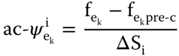

where k and q are branches, fek is the post-contingency apparent power flow, fekpre-c is the pre-contingency apparent power flow, and ΔSi is the change of apparent power injection in bus i.
Then, the SDFs are calculated based on the probabilistic attributes represented by the mean and standard deviation of all MC-based DFs (i.e., ISFs and LODFs, respectively):

where ac-DFjk is the distribution factor (ISF or LODF) of branch k provoked by contingency j (i.e., variation of power injection or branch outage), and n is the number of scenarios (m).
Since ac-DFs directly depend on each operating scenario, the complete set of short-term possible scenarios have to be previously filtered in order to improve the accuracy of SDFs (i.e., more representative mean and lower standard deviation), with the aim of obtaining more robust results. In this connection, two types of scenario filters are proposed in [23]: (i) to establish representative clusters of scenarios depending on operating similitudes, and (ii) to reduce the sample of scenarios to those with the highest probability of overload.
Once SDFs have been calculated, a table for real-time implementation has to be structured. This table includes the computed SDFs, structuring a three-dimensional matrix (or table) whose dimensions represent: (i) the branch that shows the power flow sensitivity, (ii) the type and location of the contingency, and (iii) the clusters of scenarios. For real-time applications, a classifier has to be capable of orienting the selection of the best SDFs considering the pre-contingency operating state (that can be obtained from a SCADA/EMS) and the actual contingency (that can be quickly alerted by local IEDs) [23].
After a contingency occurs, re-distributed flows (post-contingency steady state power flow fek) are estimated in each branch using the corresponding SDFs selected from the table depending on the SVC classification results, as follows:

Since there are, in general, three categories of power transfer limits: thermal, angle stability, and voltage, branch overload threshold values have to be pre-defined for each system [23]. Thus, it is necessary to pre-establish the power transfer limit (restricted by one or more of the three limits) corresponding to each element of the system. Then, an overload risk band, with upper and lower limits (Supper and Slower), can be structured in order to calculate an overload index (OVI) [23]. Therefore, once the re-distributed flows are estimated, an overload index (OVI) can be calculated for each branch using the function defined by (6.15):

where Supper and Slower are the upper and lower limits of the overload risk band for each grid element.
Then, the OVI for each electrical area is determined as follows:
For illustrative purposes, a MC-based contingency analysis simulation of the 39 bus test system, consisting of 10 000 different operating states, has been performed. The output constitutes the pre and post-contingency AC power flow results, which are used to calculate the corresponding ac-DFs. Based on the MC results and the pre-defined overload risk bands, the most critical branches are established. In this case, twelve edges present risk of overload, and these are the critical branches for which SDFs have to be calculated. After analysis, six clusters of operating scenarios have been defined for which the SDFs are computed, getting a maximum std{ac-DF} of 0.1. In the cases where SDFs are not computed, the variation of power flow does not surpass the filter limit, so it does not provoke overloads; hence the corresponding SDFs are not included in the SDF-table for real-time assessment. In these cases, the OVIs are automatically set to zero. Table 6.4 shows some of the computed SDFs (i.e., mean{ac-DF}) that correspond to different branch outages.
Table 6.4 SDFs resulting from branch outages
| Outage | Branch | Cluster / SDF (mean{ac-DF}) | |||||
| Branch (eq) | (ek) | 1 | 2 | 3 | 4 | 5 | 6 |
| L15-16 | L03-04 | 0.793 | 0.809 | 0.792 | 0.812 | 0.798 | - |
| L01-02 | L03-04 | 0.664 | 0.706 | 0.709 | - | 0.645 | - |
| L22-23 | L23-24 | 0.317 | 0.399 | 0.185 | - | 0.265 | - |
| T06-31 | L21-22 | 0.014 | 0.008 | 0.359 | - | 0.349 | - |
| T06-31 | L15-16 | 0.102 | - | 0.289 | - | 0.285 | - |
| L01-02 | L15-16 | 0.331 | - | 0.325 | - | 0.308 | - |
| L04-14 | L03-04 | 0.314 | - | - | - | 0.324 | - |
| L08-09 | L15-16 | 0.352 | - | - | - | 0.337 | - |
| T10-32 | L15-16 | 0.052 | - | - | - | 0.044 | - |
| L16-24 | L21-22 | 1.029 | 1.036 | 1.036 | 1.009 | 0.975 | - |
| L16-21 | L23-24 | 1.016 | 1.017 | 1.018 | 1.003 | 1.013 | 0.988 |
| L21-22 | L23-24 | - | - | 1.009 | 0.998 | 1.006 | 0.979 |
Table 6.5 OVIs for Branch Outages—Summary of number of cases
| Branch | OVI = 0 | 0 < OVI ≤ 0.5 | 0.5 < OVI ≤ 1 | |||
| (ek) | Sim. | SDF est. | Sim. | SDF est. | Sim. | SDF est. |
| L03-04 | 234,994 | 234,993 | 6 | 7 | 0 | 0 |
| L05-06 | 234,993 | 234,993 | 7 | 7 | 0 | 0 |
| L05-08 | 234,986 | 234,983 | 14 | 17 | 0 | 0 |
| L06-07 | 234,986 | 234,986 | 14 | 14 | 0 | 0 |
| L07-08 | 235,000 | 235,000 | 0 | 0 | 0 | 0 |
| L14-15 | 234,943 | 234,945 | 57 | 55 | 0 | 0 |
| L15-16 | 233,952 | 233,959 | 972 | 965 | 76 | 76 |
| L16-17 | 233,224 | 233,226 | 1293 | 1291 | 483 | 483 |
| L16-21 | 234,458 | 234,479 | 542 | 521 | 0 | 0 |
| L17-18 | 235,000 | 235,000 | 0 | 0 | 0 | 0 |
| L21-22 | 231,681 | 231,682 | 2876 | 2875 | 443 | 443 |
| L23-24 | 234,718 | 234,717 | 282 | 283 | 0 | 0 |
In real-time, after a contingency occurs, the SDFs will estimate the possible branch overload. Once estimation has been completed, the final step is to calculate the corresponding OVIs, which permit ranking the level of system vulnerability as regards overloads. These indices might orient the selection of corrective control actions (e.g., focused load shedding) if needed. Table 6.5 shows a summary of the number of cases that correspond to three OVI ranges. Most of the cases show excellent accuracy in estimation, mainly in the range (0.5, 1] where possible corrective control actions might be required.
6.6 Concluding Remarks
The vulnerability assessment methodology presented in this chapter allows assessing system vulnerability based on the fact that vulnerability begins to develop in specific areas of the system. In this connection, the grid is partitioned into coherent electrical areas via clustering techniques, and each one is ranked depending on several performance indices regarding vulnerability. The performance indices or indicators reflect the actual system stress level as regards five different post-contingency phenomena: transient instability, short-term voltage instability, frequency deviations outside limits (TVFS phenomena), poorly-damped power oscillations, and overloads.
Additionally, the second aspect regarding the vulnerability concept, that is the system's tendency to reach a critical state, has been included by means of a penalty into the TVFS indices (TSI, VDI, and FDI) via a scheme of logic gates.
Likewise, the possible overloads have been assessed in this chapter via an overload index (OVI). This methodology has been structured based on statistical distribution factors (SDFs), which permit the prediction of the post-contingency re-distribution of the power flow in each system branch.
On the other hand, since oscillatory stability is a slower phenomenon, its assessment does not strictly need a prediction of the future system condition. For this phenomenon, the application of modal identification techniques (such as Prony analysis) provides good enough results to giving early warning. This type of evaluation has to be performed as a complementary assessment of system vulnerability. In this connection, an oscillatory index (OSI) has been presented in this chapter.
The complete real-time post-contingency vulnerability assessment methodology depicted in this chapter gives five indicators of system vulnerability as regards different phenomena. Then, it allows identification of the phenomena involved in system vulnerability and the grid zone where the system stress is high. Therefore, this methodology might be easily used as a signal for triggering focused corrective control strategies that enable improvements in post-contingency system security.
References
- 1 U. Kerin, G. Bizjak, E. Lerch, O. Ruhle, and R. Krebs, “Faster than Real Time: Dynamic Security Assessment for Foresighted Control Actions”, 2009 IEEE Bucharest Power Tech Conference, June 28–July 2, Bucharest, Romania.
- 2 J. D. McCalley, and Fu Weihui, “Reliability of Special Protection Systems”, IEEE Transactions on Power Systems, IEEE Power & Energy Society, vol. 14, no 4, pp. 1400–1406, November 1999.
- 3 M. Amin, “Toward Self-Healing Infrastructure Systems”, Electric Power Research Institute (EPRI), IEEE, Computer, vol. 33, no 8, pp. 44–53, 2000.
- 4 I. Dobson, P. Zhang, et al, “Initial Review of Methods for Cascading Failure Analysis in Electric Power Transmission Systems”, IEEE PES CAMS Task Force on Understanding, Prediction, Mitigation and Restoration of Cascading Failures, IEEE Power Engineering Society General Meeting, Pittsburgh, PA USA July 2008.
- 5 D. McGillis, K. El-Arroudi, R. Brearley, and G. Joos, “The Process of System Collapse Based on Areas of Vulnerability”, Large Engineering Systems Conference on Power Engineering, pp. 35–40, Halifax, NS, July 2006.
- 6 Z. Huang, P. Zhang, et al, “Vulnerability Assessment for Cascading Failures in Electric Power Systems”, Task Force on Understanding, Prediction, Mitigation and Restoration of Cascading Failures, IEEE PES Computer and Analytical Methods Subcommittee, IEEE Power and Energy Society Power Systems Conference and Exposition 2009, Seattle, WA.
- 7 A. Fouad, Qin Zhou, and V. Vittal, “System Vulnerability As a Concept to Assess Power System Dynamic Security”, IEEE Transactions on Power Systems, vol. 9, no 2, May 1994, pp. 1009–1015.
- 8 J. Gimenez, and P. Mercado, “Online Inference of the Dynamic Security Level of Power Systems Using Fuzzy Techniques”, IEEE Transactions on Power Systems, vol. 22, no. 2, pp. 717–726,May 2007.
- 9 S. C. Savulescu, et al, Real-Time Stability Assessment in Modern Power System Control Centers, IEEE Press Series on Power Engineering, Mohamed E. El-Hawary, Series Editor, a John Wiley & Sons, Inc., Publication, 2009.
- 10 J. Cepeda, J. Rueda, G. Colomé, and D. Echeverría, “Real-time Transient Stability Assessment Based on Centre-of-Inertia Estimation from PMU Measurements”, IET Generation, Transmission & Distribution, vol. 8, issue 8, pp. 1363–1376, August, 2014.
- 11 J. Cepeda, J. Rueda, G. Colomé, and I. Erlich, “Data-Mining-Based Approach for Predicting the Power System Post-contingency Dynamic Vulnerability Status”, International Transactions on Electrical Energy Systems, vol. 25, issue 10, pp. 2515–2546, October 2015.
- 12 J. Cepeda, and G. Colomé, “Vulnerability Assessment of Electric Power Systems through identification and ranking of Vulnerable Areas”, International Journal of Emerging Electric Power Systems, vol. 13, issue 1, May 2012.
- 13 I. Kamwa, A. K. Pradham, G. Joos, and S. R. Samantaray, “Fuzzy Partitioning of a Real Power System for Dynamic Vulnerability Assessment”, IEEE Transactions on Power Systems, vol. 24, no. 3, pp. 1356–1365, August 2009.
- 14 J. Cepeda, J. Rueda, I. Erlich, and G. Colomé, “Probabilistic Approach-based PMU placement for Real-time Power System Vulnerability Assessment”, 2012 IEEE PES Conference on Innovative Smart Grid Technologies Europe (ISGT-EU), Berlin, Germany, October 2012.
- 15 K. Seethalekshmi, S. N. Singh, and S. C. Srivastava, “WAMS Assisted Frequency and Voltage Stability Based Adaptive Load Shedding Scheme”, IEEE PES General Meeting, Calgary, pp. 1–8, 2009.
- 16 IEEE C37.106, “Guide for Abnormal Frequency Protection for Power Generating Plants”, IEEE Power Engineering Society, 2003.
- 17 Power System Dynamic Performance Committee, Identification of Electromechanical Modes in Power Systems, IEEE Task Force Report, Special Publication TP462, June 2012.
- 18 J. Hauer, C. Demeure, and L. Scharf, “Initial Results in Prony Analysis of Power System Response Signals”, IEEE Transactions on Power Systems, vol. 5, no. 1, pp. 80–89, February 1990.
- 19 J. Rueda, C. Juárez, and I. Erlich, “Wavelet-based Analysis of Power System Low-Frequency Electromechanical Oscillations,” IEEE Transactions on Power Systems, vol. 26, no. 3, pp. 118–133, Feb. 2012.
- 20 J. Cepeda, G. Argüello, P. Verdugo and A. De La Torre, “Real-time Monitoring of Steady-state and Oscillatory Stability Phenomena in the Ecuadorian Power System”, IEEE PES Transmission & Distribution Conference and Exposition Latin America (T&D-LA), September 2014.
- 21 S. P. Teeuwsen, Oscillatory Stability Assessment of Power Systems using Computational Intelligence, Doktors der Ingenieurwissenschaften Thesis, Universität Duisburg-Essen, Germany, March 2005.
- 22 G. Amico, R. Molina, and V. Sinagra, “Rules for Determining Transmission Limits in the Power Grid of Argentina”, Proceedings of The CIGRE XII Iberian–American Regional Meeting, Foz do Iguazú, Brazil 2007.
- 23 J. Cepeda, D. Ramírez, G. Colomé, “Probabilistic-based Overload Estimation for Real-Time Smart Grid Vulnerability Assessment”, IEEE Transmission and Distribution Latin America (T&D-LA), Montevideo, Uruguay, September 2012.
- 24 J. Rossmaier, B. Chowdhury, “Further Development of the Overload Risk Index, an Indicator of System Vulnerability”, North American Power Symposium (NAPS), Starkville, MS, USA, pp. 1–6, October 2009.