
Chapter 10
Voltage Stability Enhancement by Computational Intelligence Methods
Worawat Nakawiro
Lecturer in Electrical Power Systems, Department of Electrical Engineering, Faculty of Engineering, King Mongkut's Institute of Technology Ladkrabang, Bangkok, Thailand
10.1 Introduction
Present day power systems are highly stressed conditions due to several factors such as stronger competition in generation sectors, inadequate transmission expansion [2], intermittent renewable sources and heavy use of induction machines. With these factors, a power system becomes more vulnerable to various types of unstable behaviour among which is voltage stability. This has been reported as the cause of various incidents throughout the world over the last decades, such as those in the western region (WECC) of the United States in 1996, the Chilean power system in 1997 (accounting for a loss of 80% of its total load) and the Greek system covering the whole of Athens and the neighbouring area in 2004 [1].
Voltage stability is defined as the ability to maintain an acceptable voltage profile in many parts of the system after being subject to disturbances such as gradual load increases or outages of critical lines or generating units [6]. After these events, some loads may try to restore power consumption according to their load dynamics. This may drive the weakened power system closer to the technical limits, which can lead to voltage collapse.
Several voltage stability indices have been proposed in the literature to detect proximity of the current operating condition to the voltage collapse point. These indices can be broadly categorised into model-based methods [8] and measurement-based methods [9, 10]. The former relies on approximate data and modelling of the processes of the power system. By contrast, the latter depends solely on the actual response of the power system. Reference [5] provides an extensive review of voltage stability indices and other related operational and planning aspects. In some critical situations, voltage stability has to be enhanced in order to prevent any adverse impact that could eventually lead to blackout. Preventive and corrective actions (such as in [4, 7]) can be used according to the severity of the disturbance and present state of the power system. Voltage stability constrained optimal power flow (VSCOPF) [12, 13] is an efficient tool for determining the optimal control action for the power system while ensuring sufficient stability margin in normal operation and restoring stability in critical situations. Due to the increasing complexity of the optimisation problem such as a non-convex and discontinuous search space, computational intelligence (CI) methods [14, 15] becomes an attractive tool for solving VSCOPF.
This chapter presents an application of CI methods to solve VSCOPF for preventive and corrective control actions. Ant colony optimisation (ACO) is used as the search engine in both examples. An artificial neural network (ANN) is used to provide fast estimation of the voltage stability margin (VSM) during the optimisation process in order to save computing time.
The rest of this chapter is organised as follows. Section 2 introduces voltage stability problems including key techniques for finding stability margin, namely the direct method and the continuation method [3]. In addition, the concepts of optimal power flow (OPF) and associated CI methods (namely ANN and ACO) are discussed in this section. Section 3 gives details of the IEEE-30 bus test system used in all simulations in this chapter. Section 4 presents a two-stage CI approach that guarantees minimum VSM during normal operation of the system. Section 5 explains an optimal load shedding scheme as the corrective measure to restore system stability. Corresponding simulation results are given in the respective sections. Finally the chapter is concluded and future outlook is given in Section 6.
10.2 Theoretical Background
This section reviews important theoretical concepts relevant to the method proposed in this chapter.
10.2.1 Voltage Stability Assessment
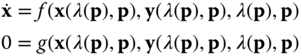
The voltage stability margin (VSM) is defined as the distance from the current operating point to the collapse point. In quasi-steady state, a power system can be modelled by a set of differential and algebraic equations

where x is the vector of state variables; y is the vector of algebraic variables and λ is a parameter that changes over time so that the power system moves from an equilibrium point to another. A vectorised form can be written as
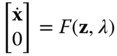
where F is the set of differential and algebraic equations and z is the vector of state and algebraic variables. It is known that the voltage collapse point corresponds to the singular bifurcation point with the following conditions:
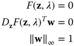
where w is the left eigenvector and Dz is the differential operator with respect to z. It should be noted that a nonlinear technique such as Newton–Raphson can be applied to solve (10.3). This method is very fast and accurate but the solution depends heavily on a good initial guess. This procedure is known as the direct method. Alternatively, one could also apply optimisation to solve (10.3) as follows:

where Δmis is the mismatch of the singularity condition and the eigenvector requirement at the collapse point.
The shortcomings of the direct method, such as a singularity near the point of collapse (POC), are overcome by the continuation method. The complete voltage profile can be generated by automatic changes of the loading parameter λ .
Figure 10.1 illustrates basic concepts of the continuation method. Assume an initial operating point (z1, λ1) lies on the curve. The so-called predictor step computes the direction vector Δz1 and the parametric change Δλ1. This gives a new point ![]() which may not lie on the trajectory. The so-called corrector step is used to ensure that the new point (z2, λ2) will lie on the trajectory. This process continues until the complete profile is obtained and the point of collapse (POC) can be located.
which may not lie on the trajectory. The so-called corrector step is used to ensure that the new point (z2, λ2) will lie on the trajectory. This process continues until the complete profile is obtained and the point of collapse (POC) can be located.

Figure 10.1 Illustration of continuation method.
10.2.2 Sensitivity Analysis
Sensitivity analysis [1] is a method used to analyse the effect of changing system parameters such as load or reactive power compensation on the stability margin of the power system. Typically change of a system parameter will cause changes to other variables. Therefore the model in (10.1) can be parameterised as
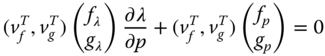
where p is the vector of changing parameters. The partial derivative due to the change of p can be written as
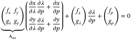
At the collapse (bifurcation point), one can find the left eigenvector ![]() corresponding to the zero eigenvalue of Asys and multiply (10.6) by this. It is obvious that the first term will vanish, leaving only
corresponding to the zero eigenvalue of Asys and multiply (10.6) by this. It is obvious that the first term will vanish, leaving only
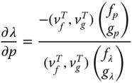
Therefore, the sensitivity of λ with respect to parameter changes is
The total change of loading margin λ due to k parameter changes can be found from the sum

This gives a linear approximation of the margin λ after the change of k system parameters.
10.2.3 Optimal Power Flow
Optimal power flow (OPF) becomes one of the important routines of modern power systems. Its objective is to achieve minimum operating cost while ensuring that constraints are within the respective limits. These limits consist of the capacity of equipment such as generators and compensating devices, security limits and stability limits. The set of optimal decision variables is determined by solving an optimisation problem with various constraints. The objective of this problem can be economic costs, system security or any other objectives. Since the early stages [20], many researchers have studied OPF with different objectives and various methods including computational intelligence [21].
Besides general objective functions of OPF such as minimisation of costs or losses, the system operator may have to assess stability of the OPF solution for all credible contingencies. If the system is unstable, the OPF solution can modified by the engineering judgement of the system operator. To guarantee optimality of the solution, the stability limit can be incorporated into the OPF software [26, 27].
10.2.4 Artificial Neural Network
An artificial neural network (ANN) is the electrical analogue of the biological neuronal system. An ANN is trained to learn the underlying relationship and perform a mapping function between the selected inputs and the outputs [19]. A typical artificial neural model is shown in Figure 10.2. A neuron is activated by the weighted sum of n inputs x1 to xn and additional bias. The intermediate output u is computed before passing through the activation function which will define the range of neural output y. Multiple neurons can be connected as a network (known as an ANN) in various configurations. Figure 10.3 shows an example of two common ANN configurations, namely feed-forward and recurrent networks. The former has no feedback from one neuron to another. This network is generally sufficient for most engineering problems. The latter is capable of handling temporal information and very suitable for predicting time series such as long-term wind speed and power [22] and solar radiation [23].

Figure 10.2 An artificial neural model.
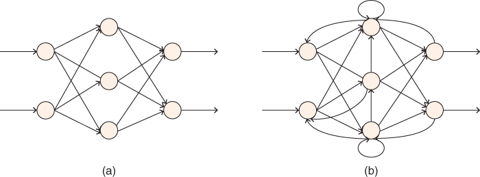
Figure 10.3 Common ANN configurations (a) feed-forward (b) recurrent networks.
10.2.5 Ant Colony Optimisation
Ant colony optimisation (ACO) is an algorithm inspired by the foraging behaviour of ants. ACO was initially developed for combinatorial optimisation problems [16]. Later, several variants of ACO emerged adapted for real-space problems, among which ACOR shows promising performance in solving test problems for unconstrained optimisation [17]. In this chapter, we have modified the ACOR algorithm to handle VSCOPF.
ACOR defines the entire search space by the weighted sum of multiple normal distributions as follows:
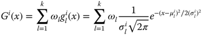
where k is the number of single Gaussian PDFs at the construction step i; ω, μ and σ are vectors of size k defining the weights, means and standard deviations associated with every individual Gaussian PDF at the construction step i.
The location of ants at each construction step represents the value of variables in real space. It is updated using a random sampling technique based on the parameters of the PDF. Unlike the pheromone trail of the classical ACO, ACOR stores the knowledge gained from previous searches in a tabular format, namely the archive XT.
Figure 10.4 shows the solution archive XT used to store n good candidate solutions that the algorithm has found so far. Since it is meant to handle the constrained problem, the quality of each solution is measured by the fitness value. Feasibility status of each solution also indicates whether the solution is desired or not. Each solution is assigned a distinct probability that the solution is chosen for the solution updating procedure of the next construction step.
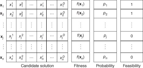
Figure 10.4 Data structure of the solution archive.
For each solution j, the weight ωj is computed from the Gaussian PDF value with mean of 1 and standard deviation of qn as
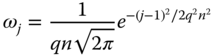
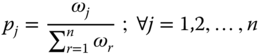
where q is a parameter of the algorithm and n is the size of solution archive. If q is small, the solutions with lower ranks in the archive have very strong influences in guiding new search directions whereby a larger q allows the wider search diversification over the entire space. For each archive solution of rank j in XT, the corresponding probability is calculated by
The new position of ant k is randomly chosen from a normal distribution again. Once the distinct selection probability is assigned to each solution, roulette wheel selection is used to select the solution which will be the mean of the distribution. The standard deviation is also computed using the average distance from the chosen solution sj to the other solutions in XT according to

where ξ is the pheromone evaporation coefficient and D is the number of variables. The position of xa becomes
where N(0,1) is the normal distribution with zero mean and unity standard deviation.
10.3 Test Power System
The IEEE 30 bus is used for all simulations in this chapter. The single line diagram is depicted in Figure 10.5.
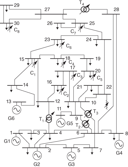
Figure 10.5 IEEE 30 bus test system.
All generators are assumed to be able to operate in under- and over-excited modes where the reactive power limits are listed in Table 10.1. Shunt reactive power sources are installed throughout the system. The limits of these sources are given in Table 10.2
Table 10.1 Generator reactive power limit (pu)
| Bus no. | 2 | 5 | 8 | 11 | 13 |
| −0.4 | −0.4 | −0.1 | −0.06 | −0.06 | |
| 0.5 | 0.4 | 0.4 | 0.24 | 0.24 |
Table 10.2 Reactive power source limits (pu)
| Bus no. | 22 | 15 | 16 | 17 | 18 | 20 | 23 | 25 | 30 |
| −0.1 | 0 | 0 | 0 | 0 | 0 | 0 | 0 | 0 | |
| 0 | 0.2 | 0.15 | 0.1 | 0.2 | 0.1 | 0.3 | 0.25 | 0.2 |
Power system simulations are carried out using the PSAT software package [24]. The MATLAB ANN toolbox [25] is used to classify stability of operating conditions and to estimate the voltage stability margin. ACO was developed as a MATLAB function.
10.4 Example 1: Preventive Measure
10.4.1 Problem Statement
In this example, a two-stage approach is developed as a preventive measure to enhance the stability margin. The first stage is to assess the stability margin of the system. If the margin is insufficient, the second stage will propose a suitable preventive control measure. Figure 10.6 shows the conceptual diagram of the proposed design. An intelligent classifier (i.e. an ANN) is trained offline so that it can inform whether or not the system has sufficient margin. For the operating conditions with insufficient margin, the optimal control parameters will be determined by solving a VSCOPF problem. The result is sent to the system operator to make the final decision.
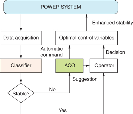
Figure 10.6 Conceptual diagram of the proposed two-stage design.
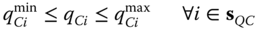
The objective of VSCOPF is to minimise transmission power loss and ensure that all security and stability parameters are within their allowable limits. Here we deal with reactive power-related variables. Therefore, the problem in this example is called voltage stability constrained optimal reactive power (VSCORPD) with the following mathematical formulation:
The constraints consist of
- a. Generator bus voltage limits
- b. Shunt compensator limits
10.17
- c. Transformer tap setting limits
- d. Load bus voltage limits
10.19

- e. Line flow limits
10.20
- f. Voltage stability margin limit
10.21

- where Ploss is the total active power losses in the transmission system; sPV is the set of generator (PV) buses; sQC is the set of shunt compensators; sT is the set of transformers; sPQ is the set of load (PQ) buses; sL is the set of transmission lines. The vector x contains control variables listed in (10.16)–(10.18) where (10.16) is treated as a continuous variable and the rest are treated as discrete variables. The vector d describes the operating condition of the power system represented by active and reactive power demand and active power generation. Note that after changing the control variables, the VSM is approximated by an offline trained ANN in order to bypass the continuation power flow procedure.
10.4.2 Simulation Results
A classifier, namely learning vector quantisation (LVQ) [18], a special type of ANN, was used to identify if the system has sufficient VSM. A dataset of 5000 samples as shown in Table 10.3 was used for training and testing. The partitioning of this dataset is given in Table 10.3 where class A contains operating points with sufficient VSM while operating points in class B have insufficient VSM and need improvement. The developed classifier shows acceptable performance on the testing dataset as shown in Table 10.4.
Table 10.3 Partitioning of dataset
| Database | Training set | Testing set |
| 5000 | 4000 | 1000 |
| Two-class partition | ||
| Class A | 1623 | 390 |
| Class B | 2377 | 610 |
Table 10.4 Performance of the classifier on testing dataset
| Class A | Class B | |
| Samples of class A (390) | 349 | 41 |
| Samples of class B (610) | 156 | 454 |
| Classification performance evaluation | ||
| Success rate | 80.3% | (803/1000) |
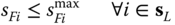
Ten operating conditions which were correctly classified as in class B are considered for voltage stability enhancement. Figure 10.7 shows that as a result of optimisation, transmission power loss is reduced significantly. Importantly, the VSM of these 10 operating points below the threshold of 25% are enhanced after VSCORPD as shown in Figure 10.8. Note that the VSM of 25% means that the system is stable with extra loadability of 25% before reaching collapse.
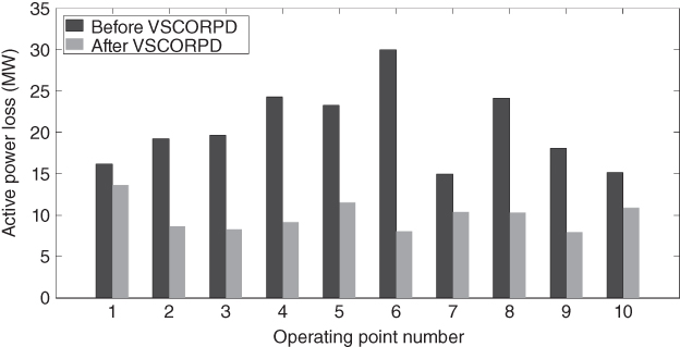
Figure 10.7 Transmission power losses.

Figure 10.8 Voltage stability margin.
10.5 Example 2: Corrective Measure
10.5.1 Problem Statement
In some serious cases, adjusting the reactive power sources is not adequate to restore system stability. Load shedding becomes an unavoidable but yet powerful option. The solution of optimal load shedding involves the determination of the effective locations and optimal amount of load to be curtailed. The former is achieved by analysing the sensitivity of load on all buses to the stability margin. However this may result in violation of some security constraints. Therefore this chapter proposes an OPF for load shedding with the objective as
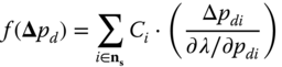
where Ci is the power interruption cost at bus i ($/kW); Δpd represents the active power load curtailment at effective buses; ![]() is the change of voltage stability margin due to the change of power demand at bus i. The constraints consist of
is the change of voltage stability margin due to the change of power demand at bus i. The constraints consist of
- a. Load bus voltage limits
10.23

- b. Line power flow limits
10.24

- where the subscripts b and m denotes the base- and maximum-loading conditions and sPQ is the set of load (PQ) buses.
- c. Fixed power factor
10.25
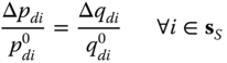
- where
 and
and  are initial active and reactive power demand of the bus i, respectively, and sS is the set of effective load buses selected for load shedding. This constraint assumed that the power factor at the selected buses remains unchanged after load shedding.
 - d. Allowable load curtailment
10.26

- e.
Voltage stability margin
10.27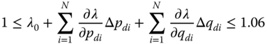
This is to ensure that the stability of the power system (λ ≥1) can be restored after the load shedding. It should be noted that a high stability margin may involve excessive load shedding. Therefore the maximum stability margin is chosen at 6%.
Table 10.5 gives the costs due to power interruption incurred by power consumers in different sectors according to [20].
Table 10.5 Power interruption cost in different sectors
| Interruption cost ($/kW) | |||
| Transportation (t) | Industrial (i) | Commercial (c) | Residential (r) |
| 16.42 | 13.93 | 12.87 | 0.15 |
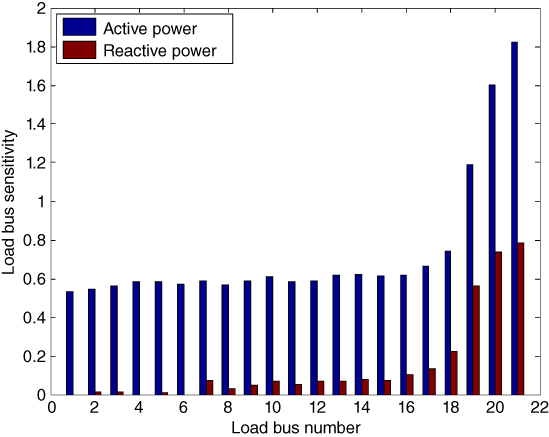
Figure 10.9 Sensitivity due to load change at different buses.
10.5.2 Simulation Results
In this example, the power system is initially voltage unstable, represented by a voltage stability margin (VSM) less than 1. Load shedding is carried out at the effective locations identified by the sensitivity analysis discussed earlier. The sensitivity of VSM due to the change of active and reactive power at load buses is shown in Figure 10.9.
Five locations are selected and their allowable ranges of load shedding are given in Table 10.6. Note that load bus numbers 17–21 correspond to buses 23, 24, 26, 29 and 30, respectively. These buses are geographically located far from the generating units and lack reactive power supports. Loads at these buses are assumed to have different configurations according to the sectors in Table 10.5. For example, the load bus 30 is of the 0.6t+0.2i+0.2r composition. This means 60% of total demand of this bus comes from the transportation (t) sector, 20% from the industrial (i) sector and 20% from the residential (r) sector. The cost of shedding 100 kW at bus 30 is $1266.8, for example. It is noted that the interruption cost at these locations is different.
Table 10.6 Information for load shedding at selected locations
| Bus | Δpdi,min(pu) | Δpdi,max(pu) | Configuration | Cost ($/100 kW) |
| 23 | 0 | 0.032 | 0.5c+0.5r | 651 |
| 24 | 0 | 0.087 | 0.3t+0.7i | 1467.7 |
| 26 | 0 | 0.035 | 1r | 15 |
| 29 | 0 | 0.024 | 0.4i+0.2c+0.4r | 820.6 |
| 30 | 0 | 0.070 | 0.6t+0.2i+0.2r | 1266.8 |

Figure 10.10 PV profile at bus 30.
Initial analysis reveals that bus 30 is the most critical one. Outage of the line between buses 28 and 27 causes a severe contingency. Figure 10.10 shows the PV profile of bus 30 after load shedding, against pre- and post-contigency (with no control actions) conditions. It is demonstrated that the proposed method is able to restore the voltage stability of the system while maintaining a number of constraints within their limits.
10.6 Conclusions
This chapter presents two examples that apply CI techniques to determine optimal preventive and corrective control measures for enhancing voltage stability of the IEEE 30-bus test system. In the first example, a combined LVQ and ACO method is proposed. The operating conditions identified to have insufficient VSM by LVQ are further analysed. Then ACO is used to determine the optimal control action that will guarantee minimum VSM. In the second example, an optimal load shedding scheme for restoring unstable operating conditions is proposed. The change in VSM due to load curtailment at effective locations is approximated by the sensitivity method in order to save computing time. Simulation results show the capability of the proposed method to improve VSM in normal operation and to restore stable operation in critical situations. Given the limited learning capability of classical ANNs when dealing with changes such as topology in power systems, further investigation on deep learning ANN is needed. Moreover, the test system used in this chapter is still not of a practical size. Selection of suitable information from a large-scale system as input features for learning purposes is of great importance.
References
- 1 V. Ajjarapu, Computational Techniques for Voltage Stability Assessment and Control. Springer Verlag, 2006.
- 2 G. Reed, J. Paserba, and P. Salavantis, “The key to resolving transmission gridlock: the case for implementing power electronics control technologies” In: Conference on electricity transmission in deregulated markets: challenges, opportunities, and necessary R&D Agenda, Pittsburgh PA, USA, pp 1–5, 2004.
- 3 C. Canizares (ed.), “Voltage stability assessment: Concepts, practices and tools” Technical Report, Special Publication of IEEE Power System Stability Subcommittee, 2002.
- 4 T. Van Cutsem and C. Vournas, Voltage Stability of Electric Power Systems. Kluwer Academic, 1998.
- 5 W. Nakawiro, “Voltage Stability Assessment and Control of Power Systems using Computational Intelligence,” Ph.D. Thesis, Faculty of Engineering, University of Duisburg-Essen, Duisburg, Germany, 2011
- 6 P. Kundur, J. Paserba, V. Ajjarapu, G. Andersson, A. Bose, C. A. Canizares, N. Hatziargyriou, D. J. Hill, A. Stankoviv, C. W. Taylor, T. Van Cutsem, and V. Vittal, “Definition and Classification of Power System Stability,” IEEE Trans. Power Syst., vol. 19, no. 2, pp. 1387–1401, May 2004.
- 7 P. Kundur, Power System Stability and Control. McGraw-Hill, 1994.
- 8 P. Kessel and H. Glavitsch, “Estimating the Voltage Stability of a Power System,” IEEE Trans. Power Delivery, vol. PWRD-1, no. 3, pp. 346–352, July 1986.
- 9 K. Vu, M. Begovic, D. Novosel, and M. M. Saha, “Use of Local Measurements to Estimate Voltage Stability Margin,” IEEE Trans. Power Syst., vol. 14, no. 3, pp. 1029–1035, Aug. 1999.
- 10 B. Milosevic and M. Begovic, “Voltage Stability Protection and Control using a Wide-Area Network of Phasor Measurements,” IEEE Trans. Power Syst., vol. 18, no. 1, pp. 121–127, Feb. 2003.
- 11 I. Simon, G. Verbic, and F. Gubina, “Local Voltage-Stability Index Using Tellegen's Theorem,” IEEE Trans. Power Syst., vol. 21, no. 3, pp. 1267–1275, Aug. 2006.
- 12 S. Kim et al., “Development of voltage stability constrained optimal power flow (VSCOPF),” Power Engineering Society Summer Meeting, 2001, Vancouver, BC, Canada, 2001, pp. 1664–1669 vol. 3.
- 13 W. Zhang, F. Li, and L. M. Tolbert, “Voltage stability constrained optimal power flow (VSCOPF) with two sets of variables (TSV) for reactive power planning,” Transmission and Distribution Conference and Exposition, 2008. T&D. IEEE/PES, Chicago, IL, 2008, pp. 1–6.
- 14 R. Eberhart and Y. Shi, Computational Intelligence. MA, USA: Morgan Kaufmann, 2007.
- 15 A. Konar, Computational Intelligence: Principles, Techniques and Applications. Heidelberg: Springer Verlag, 2005.
- 16 M. Dorigo, V. Maniezzo, and A. Colorni, “The Ant System: Optimization by a Colony of Cooperating Agents,” IEEE Trans. Syst. Man and Cybern. Part B-Cybernatics, vol. 26, no. 1, pp. 1–13, 1996.
- 17 K. Socha and M. Dorigo, “Ant Colony Optimization for Continuous Domains,” Euro. J. of Oper. Res., vol. 185, pp. 1155–1173, 2008.
- 18 T. Kohonen, Self-Ogranization and Associative Memory, 2nd edn. Berlin: Springer, 1988.
- 19 C. M. Bishop, Neural Networks for Pattern Recognition. Oxford, UK: Oxford University Press, 2007.
- 20 H. W. Dommel and W. F. Tinney, “Optimal Power Flow Solutions,” IEEE Trans. Power App. Syst., vol. PAS-87, no. 10, pp. 1866–1876, Oct. 1968.
- 21 M. R. AlRashidi and M. E. El-Hawary, “Applications of Computational Intelligence Techniques for Solving the Revived Optimal Power Flow Problem,” Elect. Power Syst. Res., vol. 79, pp. 694–702, 2009.
- 22 T. G. Barbounis, J. B. Theocharis, M. C. Alexiadis and P. S. Dokopoulos, “Long-Term Wind Speed and Power Forecasting Using Local Recurrent Neural Network Models,” in IEEE Transactions on Energy Conversion, vol. 21, no. 1, pp. 273–284, March 2006.
- 23 G. Capizzi, C. Napoli, and F. Bonanno, “Innovative Second-Generation Wavelets Construction With Recurrent Neural Networks for Solar Radiation Forecasting,” in IEEE Transactions on Neural Networks and Learning Systems, vol. 23, no. 11, pp. 1805–1815, Nov. 2012.
- 24 F. Milano, L. Vanfrett, and J. C. Morataya, “An Open Source Power System Virtual Laboratory: The PSAT Case and Experience,” IEEE Trans on Education, vol. 51, no. 1, pp. 17–23, Feb. 2008.
- 25 Mathwork Inc., “Neural Network Toolbox”, R2015a
- 26 H. R. Cai, C. Y. Chung, and K. P. Wong, “Application of Differential Evolution Algorithm for Transient Stability Constrained Optimal Power Flow,” IEEE Trans. Power Syst., vol. 23, no. 2, pp. 719–728, May 2008.
- 27 D. Gan, R. J. Thomas, and R. D. Zimmermann, “Stability-Constrained Optimal Power Flow,” IEEE Trans. Power Syst., vol. 15, no. 2, pp. 535–540, May 2000.
- 28 P. J. Balducci, J. M. Roop, L. A. Schienbein, J. G. Desteese, and M. R. Weimar, “Electrical power interruption cost estimates for individual industries, sectors and U.S. economy,” Pacific Northwest National Lab Feb. 2002.