5.6. Application to Computer Vision Problems

Thus far, we have demonstrated the capability of the tensor voting framework to group oriented and unoriented tokens into perceptual structures, as well as to remove noise. In practice, however, we rarely have input data in the form we used for the examples of sections 5.3.5 and 5.4.4, except maybe for range or medical data. In this section, the focus is on vision problems, where the input is images, while the desired output varies from application to application, but is some form of scene interpretation in terms of objects and layers.

The missing piece that bridges the gap from the images to the type of input required by the framework is a set of application-specific processes that can generate the tokens from the images. These relatively simple tools enable us to address a variety of computer vision problems within the tensor voting framework, alleviating the need to design software packages dedicated to specific problems. The premise is that solutions to these problems must comprise coherent structures that are salient due to the nonaccidental alignment of simpler tokens. The fact that these solutions might come in different forms, such as image segments, 3D curves, or motion layers, does not pose an additional difficulty to the framework, since they are all characterized by nonaccidentalness and good continuation. As mentioned in Section 5.1.1, problem-specific constraints can easily be incorporated as modules into the framework. For instance, uniqueness along the lines of sight can be enforced in stereo after token saliencies have been computed via tensor voting.

The remainder of this section demonstrates how stereo and motion segmentation can be treated in a very similar way within the framework, with the only difference being the dimensionality of the space. Stereo processing is performed in 3D, either in world coordinates if calibration information is available or in disparity space. Motion segmentation is done in a 4D space with the axes being the two image axes, x and y, and two velocity axes, v_x and v_y, since the epipolar constraint does not apply and motion can occur in any direction.

Four modules have been added to the framework tailored to the problems of stereo and motion segmentation: the initial matching module that generates tokens based on potential pixel correspondences; the enforcement of the uniqueness constraint, since the desired outputs are usually in the form of a disparity or velocity estimate for every pixel; the "discrete densification" module that generates disparity or velocity estimates at pixels for which no salient token exists; and the integration of monocular cues for discontinuity localization.

5.6.1. Initial matching

The goal of the initial matching module is the generation of tokens from potential pixel correspondences. Each correspondence between two pixels in two images gives rise to a token in the 3D (x, y, d) space in the case of stereo, where d is disparity, or in the 4D (x, y, v_x, v_y) space in the case of visual motion, where v_x and v_y are the velocities along the x- and y-axes. The correctness of the potential matches is assessed after tensor voting, when saliency information is available. Since smooth scene surfaces generate smooth layers in 3D or 4D, the decisions on the correctness of potential matches can be made based on their saliency.

The problem of matching is fundamental for computer vision areas dealing with more than one image and has been addressed in a variety of ways. It has been shown that no single technique can overcome all difficulties, which are mainly caused by occlusion and lack of texture. For instance, small matching windows are necessary to estimate the correct disparity or velocity close to region boundaries, but they are very noisy in textureless regions. The opposite is true for large windows, and there is no golden mean solution to the problem of window size selection. To overcome this, the initial matching is performed by normalized cross-correlation using square windows with multiple sizes. Since the objective is dense disparity and velocity map estimation, we adopt an area-based method and apply the windows to all pixels. Peaks in the cross-correlation function of each window size are retained as potential correspondences. The emphasis is toward detecting as many correct correspondences as possible, at the expense of a possibly large number of wrong ones, which can be rejected after tensor voting.

The candidate matches are encoded in the appropriate space as ball tensors, having no bias for a specific orientation, or as stick tensors, biased toward locally fronto-parallel surfaces. Since the correct orientation can be estimated with unoriented inputs, and moreover, a totally wrong initialization with stick tensors would have adverse effects on the solution, we initialize the tokens with ball tensors. Even though the matching score can be used as the initial saliency of the tensor, we prefer to ignore it and initialize all tensors with unit saliency. This allows the seamless combination of multiple matchers, including noncorrelation-based ones. The output of the initial matching module is a cloud of points in which the inliers form salient surfaces. Figure 5.26 shows one of the input images of the stereo pair and the initial matches for the "Venus" data set from [57]).

5.6.2. Uniqueness

Another constraint that is specific to the problems of stereo and motion is that of uniqueness. The required output is usually a disparity or velocity estimate for every pixel in the reference image. Therefore, after sparse voting, the most salient token for each pixel position is retained and the other candidates are rejected. In the case of stereo, we are interested in surface saliency, since even thin objects can be viewed as thin surface patches that reflect light to the cameras. Therefore, the criterion for determining the correct match for a pixel is surface saliency λ₁ - λ_2. In the case of visual motion, smooth objects in the scene that undergo smooth motions appear as 2D "surfaces" in the 4D space. For each (x, y) pair, we are interested in determining a unique velocity [v_x v_y], or, equivalently, we are looking for a structure that has two tangents and two normals in the 4D space. The appropriate saliency is λ₂ - λ₃, which encodes the saliency of a 2D manifold in 4D space. Tokens with very low saliency are also rejected, even if they satisfy uniqueness, since the lack of support from the neighborhood indicates that they are probably wrong matches.

5.6.3. Discrete densification

Due to failures in the initial matching stage to generate the correct candidate for every pixel, there are pixels without disparity estimates after the uniqueness enforcement module (Figure 5.27a). In 3D, we could proceed with a dense vote and extract dense surfaces as in Section 5.4.3. Alternatively, since the objective is a disparity or velocity estimate for each pixel, we can limit the processing time by filling in the missing estimates only, based on their neighbors. For lack of a better term, we call this stage discrete densification. With a reasonable amount of missing data, this module has a small fraction of the computational complexity of the continuous alternative and is feasible in 4D or higher dimensions.

The first step is the determination of the range of possible disparities or velocities for a given pixel. This can be accomplished by examining the estimates from the previous stage in a neighborhood around the pixel. The size of this neighborhood is not critical and can be taken equal to the size of the voting neighborhood. Once the range of the neighbors is found, it is extended at both ends to allow the missing pixel to have disparity or velocity somewhat smaller or larger than all its neighbors. New candidates are generated for the pixel with disparities or velocities that span the extended range just estimated. Votes are collected at these candidates from their neighbors as before, but the new candidates do not cast any votes. Figure 5.27b shows the dense disparity map computed from the incomplete map of Figure 5.27a.

The incomplete map of Figure 5.27a shows that most holes appear where the image of Figure 5.26a is textureless, and thus the initial matching is ambiguous. The discrete densification stage completes missing data by enforcing good continuation and smoothly extending the inferred structures. Smooth continuation is more likely when there are no cues, such as image intensity edges, suggesting otherwise.

5.6.4. Discontinuity localization

The last stage of processing attempts to correct the errors caused by occlusion. The input is a set disparity or motion layers produced by grouping the tokens of the previous stage. The boundaries of these layers, however, are not correctly localized. The errors are due to occlusion and the shortcomings of the initial matching stage. Occluded pixels that are visible in one image only very often produce high matching scores at the disparity or velocity of the occluding layer. For example, point A, which is occluded in the left image of Figure 5.28, appears as a better match for B' in the right image than does B, which is the correct match. Also, the difference in the level of texture in two adjacent regions, in terms of contrast and frequency, can bias the initial matching toward the more textured region.

Since it is hard to detect the problematic regions during initial matching, we propose a postprocessing step to correct such errors, which was first published in [48] for the case of motion. Since binocular cues are unreliable next to layer boundaries due to occlusion, we have to resort to monocular information. A reasonable assumption is that the intensity distributions of two surfaces that are distant in the scene, but appear adjacent from a particular viewpoint, should be quite different. Therefore, the presence of a discontinuity in the scene should also be accompanied by an edge in the image. Instead of detecting edges in the entire image and having to discriminate between true discontinuities and texture edges, we propose to focus on "uncertainty zones" around the boundaries inferred at the previous stage. The width of the uncertainty zones depends on the half-size of the matching window, since this is the maximum surface overextension as well as the width of the occluded region, which can be estimated from the difference in disparity or velocity at the boundary. In practice, we mark as uncertain the entire occluded area extended by half the size of the maximum matching window on either side.

Once the uncertainty zones have been labeled as such, we look for edges in them rather than in the entire image. This is done by tensor voting in 2D, since some of the edges we are looking for may be fragmented or consist of aligned edgels of low contrast. The initialization is performed by running a simple gradient operator and initializing tokens at each pixel position as stick tensors whose orientation is given by the gradient and whose saliency is given by

Equation 5.13

where G(x,y) is the magnitude of the gradient at (x, y), x_o is the position of the original layer boundary, and σ_e is a function of the width of the uncertainty zone. The exponential term serves as a prior that biases the extracted edges toward the original layer boundaries and, more importantly, toward the direction of the original boundaries. That is, a vertical boundary is more salient in a region where an almost vertical boundary was originally detected. This makes the edge detection scheme more robust to texture edges of different orientations. Voting is performed in 2D with these tokens as inputs, and edges are extracted starting from seeds, tokens with maximum curve saliency, and grown. Voting enables the completion of fragmented edges while the interference by spurious strong responses of the gradient is not catastrophic. Results for the example of Figure 5.28 can be seen in Figure 5.29.

5.6.5. Stereo

We pose the problem of stereo as the extraction of salient surfaces in 3D disparity space. After the initial matches are generated, as described in Section 5.6.1, the correct ones, which correspond to the actual disparities of scene points, form coherent surfaces in disparity space, which can be inferred by tensor voting. The initial candidate matches are encoded as balls, and tensor voting is performed. Then, the uniqueness constraint is enforced and tokens with low saliency are rejected as outliers. The advantage of the tensor voting-based approach is that interaction among tokens occurs in 3D instead of the 2D image space or the 1D epipolar line space, thus minimizing the interference between points that appear adjacent in the image but are projections of distant points in the scene. The output at this stage is a sparse disparity map, which for the Venus example can be seen in Figure 5.26c. Preliminary results on binocular stereo, before the development of many of the modules presented here, have been published in [34, 35].

Discrete densification is performed to fill in the holes of the sparse depth map. The results for the "sawtooth" data set of [57] can be seen in Figure 5.30c. Errors mostly exist near depth discontinuities (Figure 5.30d, where errors greater than one disparity level are marked in black and errors between one-half and one disparity level are marked in gray), and they are corrected according to Section 5.6.4. The final disparity and error maps appear in Figure 5.30e and f. Other results can be seen in Figures 5.31 and 5.32. Note that in the last example, the surfaces are not planar and the images are rather textureless. Despite these difficulties, we can infer the correct surfaces according to Section 5.4.3, which are shown texture-mapped in disparity space in Figure 5.32c-d.

5.6.6. Multiple view stereo

We have also applied the stereo algorithm to the problem of multiple view stereo. The novelty of our approach is the processing of all views simultaneously instead of processing them pairwise and merging the results. The algorithm and results can be found in [42]. The additional difficulty stemming from the increase in the number of views is a considerable increase in the number of tokens that need to be processed. Methods that operate on maps are not applicable, since uniqueness with respect to a grid does not hold in this case. This poses no additional difficulties for our method, since our representation is object-centered and not view-centered.

Candidate matches are generated from image pairs, as in the binocular case, and are reconstructed in 3D space using the calibration information that needs to be provided. If two or more candidate matches fall in the same voxel, their saliencies are added, thus making tokens confirmed by more views more salient. The number of tokens is a little below 2 million for the example in Figure 5.33. Processing of large data sets is feasible due to the local nature of the voting process. Tensor voting is performed on the entire set of candidate matches from all images, and then uniqueness is enforced with respect to rays emanating from pixels in the images. Four of the 36 input frames of the lighthouse sequence, a view of the candidate matches, and the inferred surface inliers and boundaries can be seen in Figure 5.33.

5.6.7. Visual motion from motion cues

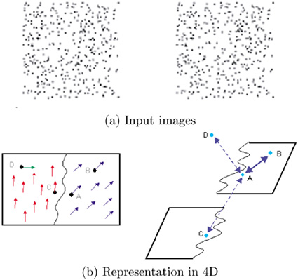
In this section, we address the problem of perceptual organization using motion cues only, which was initially published in [46]. The input is a pair of images, such as the ones in Figure 5.34a, where monocular cues provide no information, but when viewed one after another, human observers perceive groupings based on motion. In the case of Figure 5.34a the perceived groups are a translating disk and a static background. As discussed in the introduction of Section 5.6, the appropriate space in the case of visual motion is 4D, with the axes being the two image axes and the two velocity axes v_x and v_y. Processing in this space alleviates problems associated with pixels that are adjacent in the image but belong in different motion layers. For instance, pixels A and B in Figure 5.34b that are close in image space and have similar velocities are also neighbors in the 4D space. On the other hand, pixels A and C that are neighbors in the image but have different velocities are distant in 4D space, and pixel D, which has been assigned an erroneous velocity, appears isolated.

Candidate matches are generated by assuming every dot in the first image corresponds to every other dot within a velocity range in the other image. A 3D view (where the v_y component has been dropped) of the point cloud generated by this process for the images of Figure 5.34a can be seen in Figure 5.35a where v_y is not displayed. The correct matches form salient surfaces surrounded by a large number of outliers. The surfaces appear flat in this case because the motion is a pure translation with constant velocity. These matches are encoded as 4D ball tensors and cast votes to their neighbors. Since the correct matches form larger and denser layers, they receive more support from their neighbors and emerge as the most salient velocity candidates for their respective pixels. The relevant saliency is 2D surface saliency in 4D, which is encoded by λ₂ - λ₃ (see also Section 5.6.2). This solves the problem of matching for the dots of the input images. The estimated sparse velocity field can be seen in Figure 5.35b.

People, however, perceive not only the dots as moving but also their neighboring background pixels, the white pixels in the examples shown here. This phenomenon is called motion capture and is addressed at the discrete densification stage, where velocity candidates are generated for all pixels without velocity estimates based on the velocities of their neighbors. Votes are collected at these candidates, and the most salient are retained. Finally, the tokens that have been produced by both stages are grouped into smooth motion layers in 4D space. Regions and boundaries can be seen in Figure 5.35c and d. An example with nonrigid motion can be seen in Figure 5.36, where a disk is undergoing an expanding motion.

5.6.8. Visual motion on real images

After demonstrating the validity of our approach on synthetic data, we applied it to real images [45, 47, 48]. Candidate matches are generated by multiple cross-correlation windows applied to all pixels, as in the case of stereo, but since the epipolar constraint does not hold, the search for matches is done in 2D neighborhoods in the other image. The tokens are initialized as 4D ball tensors, and tensor voting is performed to compute the saliency of the tokens. The token with the largest surface saliency is selected as the correct match for each pixel after outliers with low saliency are removed from the data set. Results on the Yosemite sequence, which is a typical benchmark example for motion estimation for which ground truth exists, can be seen in Figure 5.37. The average angular error is 3.74 degrees with standard deviation 4.3 degrees with velocities computed for 100% of the image. Somewhat smaller errors have been achieved by methods that compute velocities for less than 10% of the pixels [47].

Since the input is real images, the problems described in Section 5.6.4 decrease the quality of the results, as can be seen in Figure 5.38c-d. Discontinuity detection as in Section 5.6.4 and [48] is performed to correct the velocity maps produced after discrete densification. Results can be seen in Figures 5.39 and 5.40.