
18. A Technical Explanation of Forecasting Systems
This section represents the forecast systems used in the corporate environment to add greater productivity to the corporation. Forecasting is very important in the new collaborative era. As companies are becoming increasingly interconnected, it is more important to fine-tune the forecast. The more accurate the system is, the less variance there is in creating in the entire supply chain. Because of connectivity and real-time information, decreased accuracy in-house decreases the accuracy of the collaborative partners as well. This creates a cascading effect all the way down the supply chain. This is why there is a lot of time spent on the forecasting methodologies. For example, in Six Sigma and Lean the enemy of the process is variation.
The chapter is technical in nature. The forecasting algorithms have been improved to allow the corporation to achieve an even better level of service and increased turns for the customer. The list of forecasting techniques is varied because the system is not used only to predict demand. Algorithms predict promotions, the effects of advertising, site selection, target marketing, and economic growth in different regions. The final classification of the general models used is as follows, and the forecast systems can be grouped into the following categories:
• The Algebraic Model, which includes the Multivariate Regression Model
• Trigonometric Models
• The Logistics Model
• The Logarithmic Models
• Exponential Smoothing Models, which include the Horizontal, Trend, Seasonal, and Trend Seasonal Models
The rest of the chapter explains the analysis of the variance in the forecast system. This is found in the “Dispersion of Demand” section. The chapter ends with an example of each type of exponential smoothing in the “Finding the Correct Forecast Model” section.
• The Algebraic Models and the Multivariate Regression Models are basically the same as far as the R2 and multivariate coefficients. The only difference was that they were developed for different purposes. The Algebraic Models were developed from the SAS software for predicting the promotional forecast of sale circulars. Promotions are the Achilles heel of the supply chain system, and this gives outstanding accuracy in predicting the promotional quantity needed per item for each sale. The Multivariate Regression Models were developed from the use of Minitab software. This system was used in predicting target marketing and categorical management.
• The next models presented are the Trigonometric Models used in some software packages as an alternative to seasonal forecasting.
• The Logistics Model is used to associate the advertising effect on sales revenue.
• The Logarithmic Model is used to predict new item introduction, new category introduction, or the effect of fads.
• The next series of models, which are the Exponential Smoothing Models, are used for the forecasting systems in a time series environment.
The Algebraic Model
The Algebraic Model allows the expression of forecast as a function of an independent variable multiplied by a coefficient. This forecast can be represented as a sum of the independent variables with different exponents. An example of this is Q0 = X1 * d1 + X2 * d2 + X3 * d3 + X4 * d4 + X5 * d5. The values can be determined by a good statistical package—in this case, SAS.
The number of variables will be determined by the R2 in the model. Do not add too many variables into the system because it increases the nervousness of the forecast system when too many extraneous variables are added. Using backward regression, measure the R2 of each independent variable added in. The R2 determines how much of the variation the equation explains. If the R2 measures a 43 for an independent variable, this means that the variable explains 43% of the variation when added to the equation.
To limit the number of extraneous variables, make a management policy that no one adds a variable to the forecast if it cannot explain 5% or more of the variance. This minimum percentage for R2 can change from the type of forecast needed and the management philosophy. Typically, a backward regression system will list the R2 values with the independent variable. The R2 value in a backward regression lists the variables with the highest R2 to the lowest. Always start to add the largest values of the R2 into the forecast first. For example, the system has listed the following set of values:
• R2 = 40% for X1
• R2 = 30% for X2
• R2 = 12% for X3
• R2 = 8% for X4
• R2 = 5% for X5
• R2 = 2% for X6
In the preceding case, select only the top five variables because the sixth variable has an R2 under 5%. The forecast system is represented as Q0 = X1 * d1 + X2 * d2 + X3 * d3 + X4 * d4 + X5 * d5. The values represent a new forecast for the next month. The d1 is the demand for the current month. The d2 is the demand for the last month, and the d3 is the demand for the month two periods in the past. The total explanation of the variation is 95%, which is the sum of the R2s. The forecast model typically represents the data in monthly terms to make it easier to understand. The forecast for January, run in December, is Qjan = X1 * ddec + X2 * dnov + X3 * doct + X4 * dsep + X5 * daug with an R2 of 95%. Note: The d and X values do not need to just be demand values. They can denote other events that show correlations to the dependent variable. The other conditions can help by predicting the price elasticity to demand when running a promotion. How much will sell at this price? How will the effect of increased advertising in an area increase sales? Which items should be selected in a target market?
Multivariate Regression Models
Regression Models using regression analysis can be used to infer causal relationships between the independent and dependent variables. The forecast uses external data as the independent data to represent its forecast. This approach is used to help increase the accuracy of the forecast by including external variables such as these:
• Housing starts
• Interest rates
• GDP growth
• Spendable income
• Price elasticity to demand
• Ethnic variables
• Type of home in an area
• Age in the community
The illustrated Regression Model shows three forms of forecast models. The model that predicts the demand with the greatest amount of accuracy has the least MAD or highest R2. The Regression Model uses the Minitab software. The three forms are the linear, the quadratic, and the cubic forecast models. The graphs were also drawn from the Minitab software. The regression can be linear like Y = β0X + C where β0 is the coefficient and C is the constant. This can represent a Horizontal or Trend Model in a cyclical demand pattern graphed in Figure 18-1. Note that the R2 shows a 0%, which indicates that the model does not predict the demand at all.
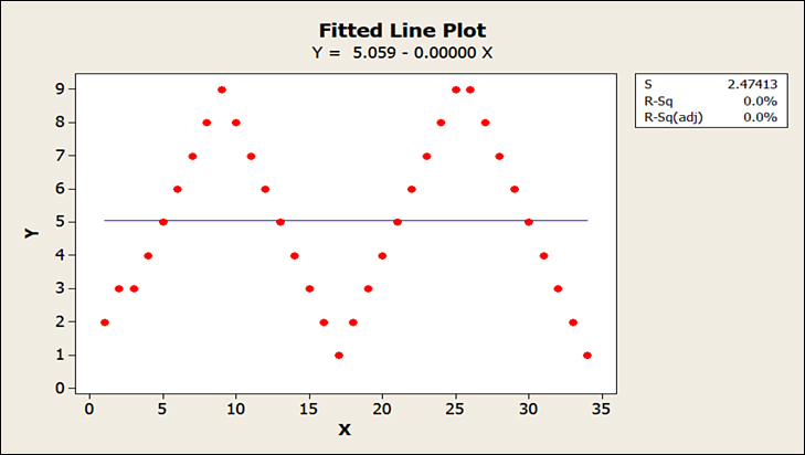
Figure 18-1. Using a Horizontal or Trend Model in a seasonal or cyclical demand pattern
It can be parabolic or to the power of two like Y = β0 X1 + β0 X22 + C. Note that the R2 shows as 8.2%, which explains that the parabolic model accounts for only 8.2% of the variation. This is illustrated in Figure 18-2, which shows the improvement over the previous model by introducing the quadratic model. This is not the appropriate model for the demand pattern. A quadratic model is used when the demand shows a maximum or minimum and turns the other direction after hitting the maximum or minimum.
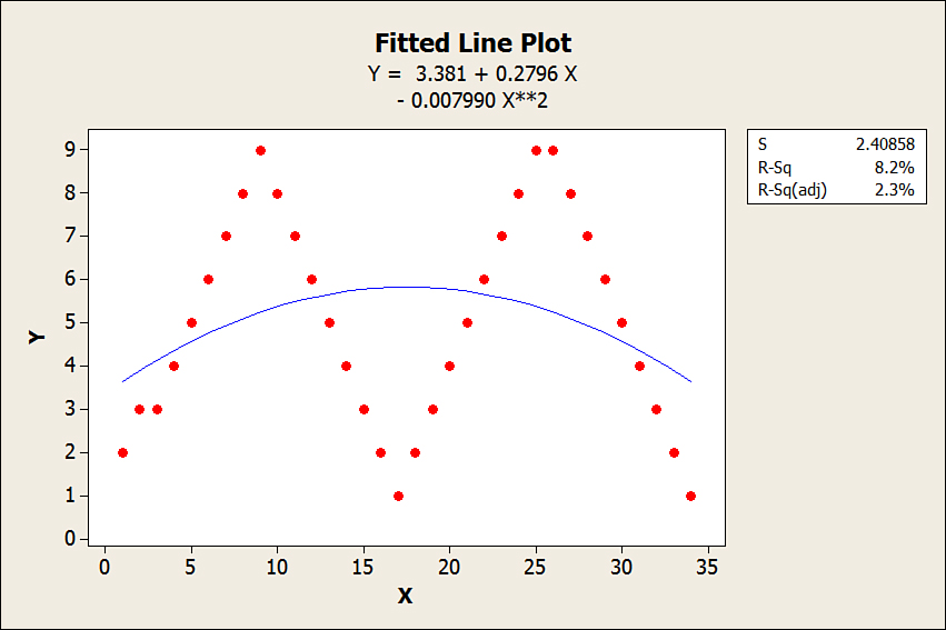
Figure 18-2. Using a Quadratic Model in a seasonal or cyclical demand pattern
Finally, it can be to the power of three known as a cubic model like Y = β0 X1 + β1 X22 + β2 X33 + C. Note that the R2 shows as 9.6%, which explains that the parabolic model only accounts for 9.6% of the variation. This is illustrated in Figure 18-3, which shows the improvement over the previous model by introducing the cubic model. This is also not the appropriate model for the demand pattern. The appropriate model would be a seasonal forecast model, as explained in the following chapter on exponential smoothing.
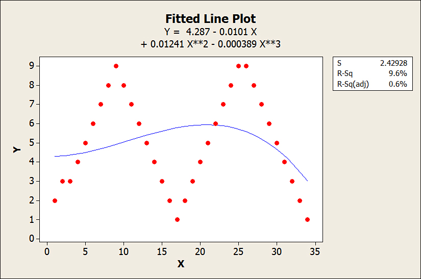
Figure 18-3. Using a Cubic Model in a seasonal or cyclical demand pattern
Trigonometric Models
As a classification, the Trigonometric Model would be the Fourier Transform. The transform could be available in the software program as an alternative to the exponential smoothed seasonal indexing model. Sometimes people use this concept versus seasonal indexing in Exponential Smoothing Models, which is discussed later in this chapter. Because the independent variable is a time value, it can be used in predicting cycles, oscillations, or seasonal cycles. Both are used to forecast seasonal or cyclical data patterns. Compare both models to see which one gives the more accurate solution. This is determined by seeing which system gives the lowest mean absolute deviation (MAD). The concept of MAD is discussed later.
The Logistics Model
The Logistics Model can be used to approximate sales and advertising. This approach measures advertising spending to actual sales increases. The advertising dollars are the independent variable and sales are the dependent variable. An example of the logistics formula would be y = a / (1 + b e-kx), k > 0. As an example using the preceding formula, the system calculates the following results:
• a = $100,000, which is the maximum reachable revenue. This means that the maximum revenue, no matter how many dollars are spent, is $100,000.
• b = 200,
• k = 1,
• e = 2.718282,
• The X axis is the increase in adverting dollars as a percentage:
• X = 1.0: No increase.
• X = 1.1: Increase advertising 10%.
• X = 1.2: Increase advertising 20%.
• X = 10.9: Increase the advertising by 10.9 times the original value.
• The graph in Figure 18-4 illustrates the effect of the Logistics Model. The top line represents sales. The bottom line represents change in advertising. This shows the relationship of advertising dollars to sales.
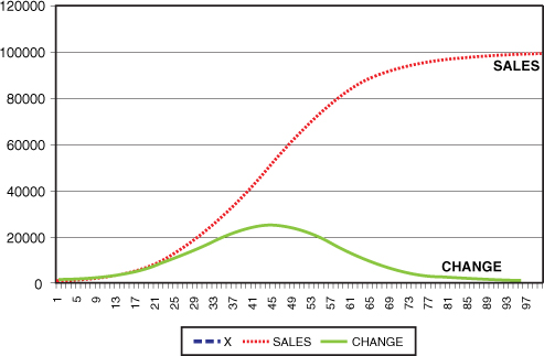
Figure 18-4. Graph showing the relationship of advertising dollars to sales
The maximum increase in sales is when adverting is increased by 45, denoted by the flattening out of the change line. At this point, the slope of the line is zero, which means you have achieved a maximum. The bottom line represents change in sales for each percentage of increase in advertising dollars. After this point, the change becomes negative. This represents a 350% increase in adverting budget. Beyond this point, returns diminish.
The Logarithmic Models
These models are used to forecast a new item introduction when it is expected to act as a fad-changer. This predicts the growth curve of the product. The Logarithmic Model has a period of rapid increase of sales, followed by a period when the growth slows. The interest is in the beginning growth portion of the graph because it is the hardest to forecast. The main difference between the models is that the Exponential Model begins slowly and then increases rapidly as time increases, whereas the Logarithmic Model begins fast and then decreases rapidly as time increases. Figure 18-5 shows the rate of increase of sales for a new item over time.

Figure 18-5. Using Logarithmic Models to model the growth curve of a new item with a = 1 and b = 40
This is the formula for the Logarithmic Model: y = a + b * ln x.
• a = 1. This is the point where the graph starts to depart from the Y axis and begins its logarithmic slope.
• b = the coefficient or percentage contribution of the ln function, and it is set to 40 in this case. As a good rule of thumb, take the b value and multiply it by 5 and the curve will cross the Y axis value at approximately the 145 period. This is significant because now there is a template in which to overlay the sales pattern. For example, if the forecast reads that the sales will be $200,000 in approximately 5 months, then use a b value of $200,000 / 5 = 40,000. The result is the higher the b coefficient, the greater the Y axis values or anticipated sales. Another rule of thumb is that as you increase b you multiply the initial growth by 6.9315. The initial growth when b is equal to 40 is 277 units sold the first month. If you set b to equal 80, then you forecast sales of 80 * 6.9315 = 555 units sold the first month. This is just another tool in using the model. If you estimate the first month’s sales, the rest of the graph can be estimates. After your first month’s sales are available, you can adjust b to match the actual first month’s sales. The adjusted graph may give a better prediction of the future months’ sales.
• x = the number of months after introduction.
• x = 1 means 1 month after introduction.
• x = 2 means 2 months after introduction.
• x = 100 means 100 months after introduction.
• The X axis shows the month after the introduction of the new item.
• The descending line shows the decline in the amount of positive change in sales over time.
• The top line is the anticipated sales over time. With a value of a = 1 the sales go above the 150 in Period 42.
• The point of diminishing returns would be around 10 to 13 months.
The effect of a on the graph is the point where the graph forms the logarithmic curve. The a value is set to 10 in Figure 18-6 and note the curve leaves the Y axis at the point of 10. In other words, it starts its sales growth at a higher level. With a value of a = 10, the sales go above the 150 in Period 34 as opposed to Period 42 in Figure 18-5.
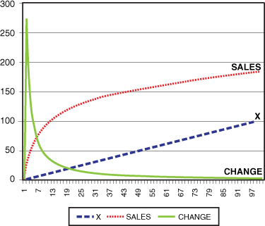
Figure 18-6. Using Logarithmic Models to model the growth curve of a new item with a = 10 and b = 40
Figure 18-7 shows when a = 100, the curve leaves the Y axis at 100. This means that the sales will begin at a higher value as opposed to using the a value of 1 or 10. With a value of a = 100 the sales go above 150 in Period 4.
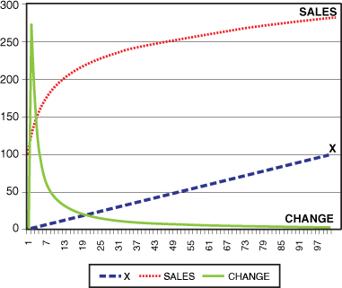
Figure 18-7. Using Logarithmic Models to model the growth curve of a new item with a = 100 and b = 40
Exponential Smoothing
Gamma smoothing is a unique contrast to exponential smoothing. Exponential smoothing is the use of a constant like α = .1 to change the forecast. Alpha α = .1 means to take 10% of the most recent data in figuring the new forecast. The formula is New Forecast = Last Forecast + .1 * (Current Demand − Last Forecast). This actually weights the importance of the most recent demand to the demand in the past. Table 18-1 shows the percentage contribution to the current demand and the past demand.
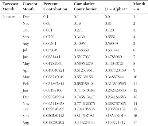
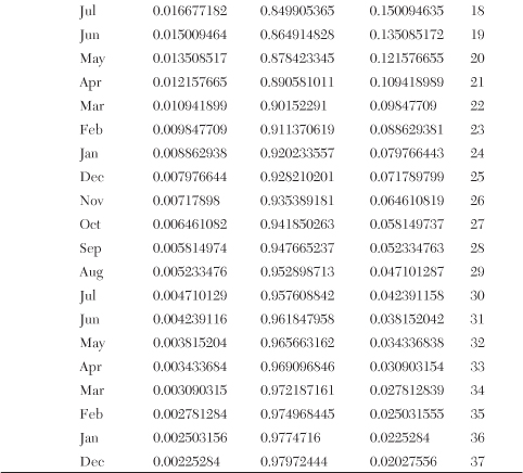
Table 18-1. Percentage Contribution
The table shows the relative importance of each month in the past to the forecast. The last month influences the forecast by 10%. The month prior shows a 9% contribution to the forecast with a total cumulative contribution for the two months of 19%. The third month shows an 8.1% contribution to the forecast with a total contribution for the three months of 27.1%. Now consider yearly numbers. With an exponential smoothing constant of .1, the last 12 months have a 71.76% influence on the forecast. The last two years will influence the forecast by 92.02%.
Changing the exponential smoothing constant can have a large effect on the amount of planning horizon of the forecast. For instance, changing the alpha from .1 to .2 results in subsequent changes. The last month influences the forecast by 20%. The month prior shows a 16% contribution to the forecast with a total cumulative contribution for the two months of 36%. The third month shows a 12.8% contribution to the forecast with a total contribution for the three months of 48.8%.
Consider yearly numbers again. With an exponential smoothing constant of .2, the last 12 months have a 93.13% influence on the forecast. The last two years will influence the forecast by 99.5%. By using an exponential smoothing constant of .2, any disturbances in the first year will have a 93.13% effect on the forecast.
Changing the A constant seeks the quantity that minimizes MAD. In the last models of regression, R2 was used as a measure of fit. MAD could also have been used as a measure of fit.
Exponential Smoothing for a Horizontal Model
The Horizontal Model is the forecast of demand for a time series that does not experience trends, cyclicality, or seasonality. This is also known as single exponential smoothing.
The formula for exponential smoothing is Ft = Ft-1 + α(At-1 − Ft-1).
• Ft = new forecast for the next month.
• Ft-1 = forecast for current month.
• α = the exponential smoothing constancy and is generally .1 to .15.
• At-1 = actual demand from the current month.
The next example illustrates how it works. It starts with a current demand of 50. The example fills the numbers in to show how the exponential smoothing works in an applied fashion.
• Ft-1 = forecast for the current month = 580.
• α = .10.
• At−1 = actual demand for the current month = 700.
• Ft = Ft-1 + α(At-1 − Ft-1) = 580 + .10(700 − 580) = 580 + 12 = 592. The Ft is the forecast for the next month, which equals 592.
Figure 18-8 shows the relationship of the forecast to demand. A represents actual demand and Ft is the forecast generated from the horizontal forecast model. Note that the MAD is 94.65. Whichever model is selected should have the smallest MAD.
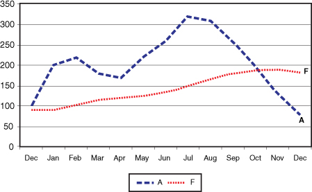
Figure 18-8. Graph of the horizontal exponential smoothing
Exponential Smoothing for a Trend Model
This is the time series model which incorporates the Trend Model. It is sometimes referred to as double exponential smoothing because it has two steps to the process and uses two smoothing constants, α and β. It is calculated as follows:
• Ft = α(At-1) + (1 − α) * (Ft-1 + Tt-1).
• β = usually 2 * α or greater depending on choice.
• Tt = β(Ft − Ft-1) + (1 − β) * Tt-1
• Step 1 is to compute Ft.
• Step 2 is to compute Tt.
• Step 3 is to calculate the forecast FITt = Ft + Tt, which represents forecast with trend.
Begin with the actual demand noted as Actual in Table 18-2. There must exist an initial forecast called F, and the initial trend to start the model has to be estimated. The trend can be estimated by inspection of the graph or simply calculated as the average amount of growth between several points. This can be represented as T. The α is the exponential constant and the β is the smoothing constant for the trend element T. It is usually twice the alpha constant. If α = .10 then β will equal .20. In this case, the β = .40. The first line with the given demand of 100 followed by the estimate of the forecast and trend begins the process. This allows you to have the initial data to begin the trend forecast.

Table 18-2. Calculating Forecast Including Trend
The graph in Figure 18-9 shows the forecast versus actual demand. The MAD is calculated as 86.39. This is lower than the Exponential Smoothing Model of 94.65. In this case, use the Trend Model. Graphically, the Trend Model shows that the forecast is closer to the actual demand compared to the Horizontal Model.
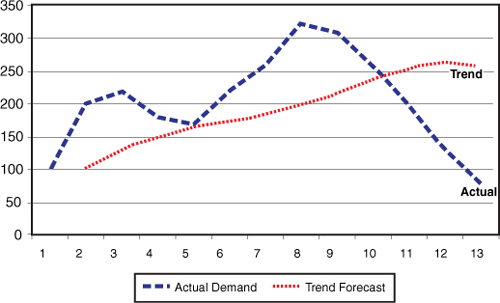
Figure 18-9. Graph of the trend exponential smoothing
Exponential Smoothing for a Seasonal Model
The seasonal model uses base indexes (BI) to calculate the forecast for future months. The indexes also give a very good idea of the seasonal profile. How is it that some months consistently sell more than or less than the other months throughout the year? At this point, average out the last three years, denoted as Avg. Now calculate the average per month for the three years. For example, take the last three January sales for each of the last three years and find the average. Do the same for February all the way to December. This is called the monthly average Mt. The reason for using the last three years’ consumption is that it averages out late or early seasonal patterns.
• Mt is the average of the monthly demand per month for three years.
• The BI = Mt/Avg.
• The Avg is the three years average of all 36 months.
• The Mt is calculated in the following table and again is all three months’ sales for each year added together and divided by three. After this is calculated, the BI base index is determined by dividing each month’s M value by the overall three-year average called Avg. Table 18-3 shows you how the base index (BI) is calculated.
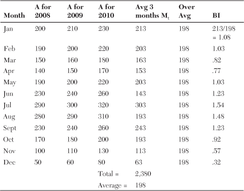
Table 18-3. Calculation of the Base Index
The next step is to determine how to forecast seasonality using exponential smoothing. As an example, in November 2010 the deseasonalized Ft was equal to 220. The deseasonalized value is the average for the month with seasonality taken out. Begin the forecast with a deseasonalized value. This is the average value for all 12 months. Find the deseasonalized value for each month. This starts by creating the base index for each month. With the base index values configured, divide the month’s actual sales by the base index to see what the demand would be for the months without any seasonal influence.
To more easily follow the development of the forecast in the following step-by-step process, a few terms need to be defined. FS stands for the seasonalized forecast created from the deseasonalized demand multiplied by the base index. FD stands for the forecast for the month deseasonalized, which is synonymous with the average demand for the year. BI is the monthly base index, synonymous with the ratio of the month’s expected demand above or below the mean. The next step is to create the new seasonal forecast, which is a two-step process:
• To create the new forecast for January, use the deseasonalized demand for December. The calculation is as follows:
FDDEC = (FSDEC + α * (ADEC − FSDEC)) / BIDEC
• The new seasonalized forecast for January is FSJAN = BIt-11 * FDDEC.
• The index t-11 used on the BI stands for the 11th month back from the current month when the current month is December. The 11th month back is January 2010. BIt-11 is the base index for January 2010 and is used to calculate the forecast for January 2011.
• FDDEC stands for December’s deseasonalized average.
• BIt-11 stands for the base index for January 2010 and is used to calculate the forecast for January 2011.
• FSJAN stands for January 2011’s seasonalized forecast average.
• Now that January’s demand is calculated, February’s forecast can be completed:
• Calculate the deseasonalized demand for January:
FDJAN = (FSJAN + α * (AJAN − FSJAN)) / BIJAN
• AJAN is the actual demand for January 2011. So the equation smoothes the difference of how far the forecast missed the actual demand. At this point, take a percentage of the miss, which is α, and add it onto the new smoothed January deseasonalized demand.
• This deseasonalized demand for January is used to compute the seasonalized demand for February. All seasonal forecasts begin with the deseasonalized demand and use the two-step approach.
• The new deseasonalized demand for February is used to calculate the March seasonalized demand forecast through the same two-step approach:
FDFEB = (FSFEB + α * (AFEB − FSFEB)) / BIFEB
FSMAR = BIT-11 * FDFEB
• Table 18-4 shows the rest of the months filled in.
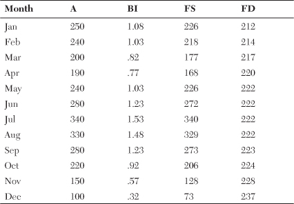
Table 18-4. Calculating the Seasonalized Demand from the Deseasonalized Demand
The chart in Figure 18-10 shows the tracking of the exponential smoothing constant and the tracking of the seasons within the time series.

Figure 18-10. The comparison of the demand pattern with the seasonal forecast.
Note the closeness in the forecast FS and the actual demand. The next operation to complete is to smooth the BI values for each month because these values can change over time.
Exponential Smoothing for a Trend Seasonal Model
Figure 18-11 highlights the trend in the forecast that we must address.

Figure 18-11. Emphasizing the trend component of the seasonal forecast
The formula for exponential smoothing, including trend, is FDT+1 = α(At) + (1 − α) * (FDt + Tt).
β is usually 2 * α or greater depending on choice. In the last example, the choice was 4 * α.
This follows a four-step process:
1. Compute FDt+1, where FDT+1 = α(At) + (1 − α) * (FDt + Tt).
2. Compute Tt+1, where Tt+1 = β(FDt+1 − FDt) + (1 − β) * Tt.
3. Calculate the forecast FITDt+1 = FDt+1 + Tt+1, which represents Forecast with trend for the next period.
4. Calculate the seasonal forecast FITST+1 = FITDt+1 * BIT-11.
An example of this forecast is as follows:
Trend Seasonal
MAD
The initial MAD is calculated as the absolute value of the demand minus the average for one year, MAD0 =
This stands for the initialized value of MAD. After this is calculated, the MAD is updated by using the following formula over time:
How much is the forecast missing the actual demand? In the beginning, the first smoothed value uses the initial estimate MAD0 to smooth against the deviation between the forecast and the actual demand or the MAD value. This value is smoothed over time as each month is tracked. Reinitialization is the time the initial values for the forecast system were calculated and then double-checked to determine whether any forecast model changes needed to be made. The MAD0 is calculating from the last 12 months. This first value gives a base to start with. After the initial MAD is calculated, the rest of the calculations for the future values are determined through exponential smoothing.
The formula for the new MAD is as follows:
MAD1 = MAD0 + α / 4 * (A0 − F0)
• MAD1 = the MAD for the next month based on the current absolute deviations.
• α / 4 = the current exponential rate used in the Horizontal Model divided by four. The alpha is divided by four to minimize the variation in the MAD calculation. If it is not divided by four, volatility is introduced into the forecast model.
• The rest of the calculations are represented by the following formula. CSFE stands for the Cumulative Sum of the Forecast Errors:
Table 18-5 shows the initialized value of the
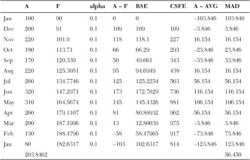
Table 18-5. The Creation of MAD Mean Absolute Deviation
With the beginning MAD in place, calculate the
Remember that a beginning forecast is not necessary but an average is.
Now that the average mean from initialization is calculated, the new MAD for future months can be determined. Consider that the MAD in the preceding chart was calculated in December. Use this value to calculate the forecast for January. At the end of January, measure the demand for that month, assumed for this example to be 150. From the initial calculation, smooth the MAD for the subsequent months. The February MAD is
AJ = 150.
α = .10.
FJ = 182.6317 forecast for January 2011 calculated in the chart.
MADJ = 56.450, which was calculated from the initialization phase.
MADF = MADJ + α / 4 * (AJ + FJ) = 56.450 + (.10 / 4) * (150 − 182.6317) = 56.3684.
The MAD for March would be calculated the same way, or MADM = MADF + α / 4 * (AF + FF). This process will calculate the MAD for each month in the time series.
Order Quantity
The order quantity calculation can vary by type of forecast model.
• Horizontal Model: OQH = Ft * (LT + RT) + k * MAD * (LT+RT).7
• Trend Model: OQT = FITt * (LT + RT) + k * MAD * (LT+RT).7
• Seasonal Model OQS is explained as follows:
• OQ = Σ(BIt-8 + BIt-9 + BIt-10 + BIt-11) * FDt-1 * (LT + RT) k * MAD * (LT+RT)7 where Σ(BIt-j) represents the number of periods or partial periods in (LT + RT).
• In forecasting the OQ in December for next year and (LT + RT) = 4, then the equation would be represented this way:
OQ = Σ(BIAPR + BIMAR+ BIFEB+ BIJAN) * FDDEC * (LT + RT) k * MAD * (LT+RT)7
• The k values are found in Table 21-1 and give the relationship of k to the Z transform. The system uses the k values for MAD, and using the standard deviation requires the use of the Z value. This is only showing the comparison for illustration.
Dispersion of Demand
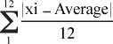
With the concept of adoptive forecasting, the alpha constant can be changed when the forecast error begins to increase. This is accomplished with the use of tracking signal trips (TS) and the Running Sum of Errors (RSE). ![]() . The RSE is the accumulative difference between the demand and the forecast for the same period. The tracking signal is tripped when it reaches a value of > 3 or < 3. The tracking signal also determines whether there is too much forecasting being done or whether the forecast is on the high or low side.
. The RSE is the accumulative difference between the demand and the forecast for the same period. The tracking signal is tripped when it reaches a value of > 3 or < 3. The tracking signal also determines whether there is too much forecasting being done or whether the forecast is on the high or low side.
The Demand Filter (DF) indicates whether the target is consistently missed on the high or low side. ![]() . When DF > 6, it will trip the Demand Filter. The Demand Filter can also calculate whether the demand is changing dramatically or the demand is an outliner. The term “outliner” is used because it is a computer program that organizes text into discreet groups. “Outliner” represents the outliers in terms of discreet numbers. An outliner is defined as a very high or low demand that does not represent the demand pattern. It is usually excluded or taken out of the calculation. In this case, ignore smoothing the variables because the demand is probably an error. The Tracking Signal with the Demand Filter will signify that closer attention must be paid to the forecast and one of the following corrective measures is necessary:
. When DF > 6, it will trip the Demand Filter. The Demand Filter can also calculate whether the demand is changing dramatically or the demand is an outliner. The term “outliner” is used because it is a computer program that organizes text into discreet groups. “Outliner” represents the outliers in terms of discreet numbers. An outliner is defined as a very high or low demand that does not represent the demand pattern. It is usually excluded or taken out of the calculation. In this case, ignore smoothing the variables because the demand is probably an error. The Tracking Signal with the Demand Filter will signify that closer attention must be paid to the forecast and one of the following corrective measures is necessary:
• Reinitialize the forecast or reevaluate the forecast model. Should it be Horizontal, Trend, Seasonal, or Trend Seasonal? If the model changes, run the reinitialization on the item to see what new model fits the demand better. During reinitialization, set the default MAD into the file. Remember, the default MAD is calculated as
After the software has selected a new model, the TS indicator should be reset to zero. It isn’t necessary to change the alpha for the Exponential Smoothing Model yet. If it still continues to trip the tracking signal limits after the forecast model has changed, begin reevaluating a change in the alpha value in the model.
• If the model stays the same, change alpha. The TS indicator will be reset to 0.
Table 18-6 shows the forecast F, FE, RSE, AFE, CAFE, TS, and DF and is used to calculate the TS tracking signal and DF Demand Filter.

Table 18-6. Forecast Through the Tracking Signal and MAD
The columns for Table 18-6 are defined here:
• F = The Forecast for the Period
• FE = Forecast Error
• RSE = Running Sum of Errors
• AFE = Absolute Forecast Error
• CAFE = Cumulative Absolute Forecast Error
• DF = Demand Filter
• TS = Tracking Signal
• MAD = Mean Absolute Deviation = CAFE/N
• N = Number of Periods Measured in the CAFE
In the table, if the tracking signal gets larger than 3 or 4, consider either reinitializing to change the forecast model or changing the alpha constant. In this case, the tracking signal is 4. In May, the TS = 4.90. This is a problem because there is a strong positive bias to the forecast that must be addressed. In some cases, there may be a few false trips with the tracking signal but each one requires further investigation.
The demand filter is used to check individual forecast errors. The amount of deviation from the demand and the forecast is divided by MAD. If the DF > 6, look at the usage as a possible outliner or potential change in demand. DF = (Demand − Forecast) / MAD. In this case, the limit for the demand filter is set for values above 3.33.
A Tracking Signal (TS) trip of 3 would signal the system to possibly change the alpha from .1 to .13. As the forecast is continually missed, the α alpha constant is changed. After the tracking signal has been tripped and the α alpha constant is changed, for example, from .1 to .13, then the TS is zeroed out and the calculation begins again. If demand starts to change, the correction will be a stepladder approach. Each time the TS is tripped it is zeroed out and then the TS must accumulate the biased errors either negative or positive before it is tripped again. One approach, if the forecast model has not been changed, is to successively increase the alpha content from .1 to .13, then .16, then .20. It is possible to extend the increase of alpha beyond this point but sometimes it brings in too much nervousness in the system.
Finding the Correct Forecast Model
Initialization is scanning the set of forecast models to find and use the correct one for each item in the warehouse. It should be noted that each item is warehouse-dependent, meaning that an item may have a different forecast model for different warehouses. Each item in the inventory will probably possess its own unique demand pattern. Some warehouses may be trend whereas others may be horizontal and a few could be seasonal.
The correct procedure to determine the model is to wait for a tracking signal trip. After the item has been tripped, it will go through the process of initialization. This process compares the MAD for each successive forecast model. The usages used in this calculation are the last year’s usage based on the smallest MAD. This visual approach is used only for demonstration. In the normal process, the computer only looks at the MAD in its quest to find the correct forecast model.
The Horizontal Exponential Smoothing Model
The first comparison is for the Horizontal Model in Table 18-7. The A represents actual demand. The F is the forecast for the period. The alpha is the smoothing constant (A − F), which represents the difference between the actual and the forecast. The calculations for the MAD follow Table 18-7. The Horizontal Forecast Model is represented by the formula Ft = Ft-1 + α(At-1 − Ft-1). The RSE represents the Running Sum of Errors. The Running Sum of Errors should net out close to 0. In this case it does not because the forecast is always below the demand. There is a trend component in the demand and the forecast is not using the horizontal model instead of the trend model. In a case like this, consider changing the forecast parameters or changing to a Trend Forecast Model. Figure 18-12 shows how the forecast does not keep up with demand because of the large gap between A (actual demand) and F (the forecast).

Table 18-7. Exponential Smoothing Including Horizontal and Trend

Figure 18-12. Demand versus forecast for the Horizontal Model
The MAD from these values is 94.65898.
The Trend Exponential Smoothing Model
The next comparison is for the Trend Model. The A represents actual demand. The FIT is the forecast including trend for the period. The alpha is the smoothing constant. A − F is the difference between the actual and the forecast including trend. The MAD is calculated for the Trend Model in Table 18-8.
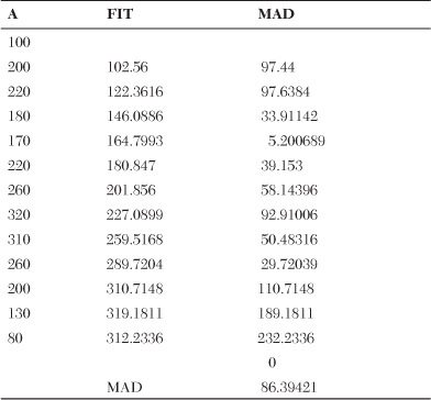
Table 18-8. The Calculation of MAD from a Trend Model
The graph in Figure 18-13 represents the actual demand and forecast for the Trend Model. Note that the MAD for the Trend Model is 86.394, which is 8.2647 lower than the Horizontal Model’s MAD of 94.65898. This is an improvement over the Horizontal Model. It’s noted that the gap between the actual and the forecast is greater for the Horizontal Model. As the MAD becomes smaller, the gap between the actual demand and the forecast becomes smaller.
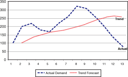
Figure 18-13. Demand versus FIT (forecast including trend) for the Trend Model
The Seasonal Exponential Smoothing Model
The final comparison is for the Seasonal Model. The A 2010 represents actual demand. The FS2 is the forecast seasonalized by the use of base-index values. The alpha is the smoothing constant. The MAD calculations for the seasonal model are performed shown in Table 18-9.
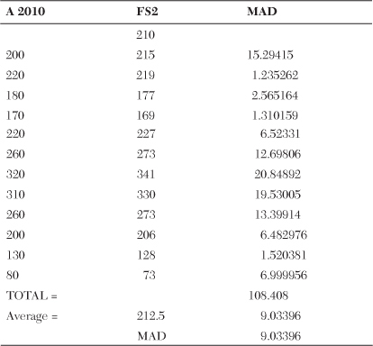
Table 18-9. The Calculation of MAD in a Seasonal Model
The graph shown in Figure 18-14 is the actual demand and forecast for the Trend Model. Note that the MAD for the Trend Model is 86.3942. The Seasonal Model is 77.3602, which is 9.034 lower than the Trend Model. This is a large improvement over the Trend Model. In comparing the two graphs, note that the FS tracks the peaks and values of the demand. This is why the MAD is much lower for the seasonal forecast.
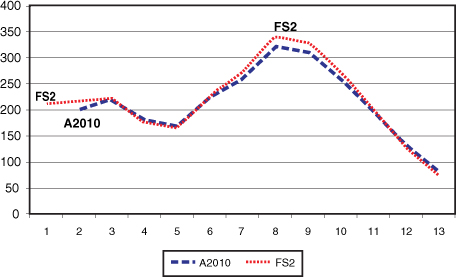
Figure 18-14. Demand versus forecast using the Exponential Smoothing Seasonal Model