7.1.1 Definition of Cultural Heritage

Cultural heritage is the legacy of physical artifacts and intangible attributes of society inherited from past generations. Physical artifacts include works of art, literature, music, archaeological and historical artifacts, as well as buildings, monuments, and historic places, whilst intangible attributes comprise social customs, traditions, and practices often grounded in aesthetic and spiritual beliefs and oral traditions. Intangible attributes along with physical artifacts characterize and identify the distinctiveness of a society.

Small artifacts such as sculptures, pottery, coins, armor, paintings, etc., are preserved in museums and art galleries. Buildings, monuments, and historic places are often subject to preservation orders and regulation by government to ensure their survival for future generations. Cultural heritage artifacts are to a greater or less extent unique and irreplaceable. This poses a number of economic questions beyond the immediate question of how much are people willing to pay to consume (use, see, experience) different cultural goods. How much are people willing to pay to preserve cultural heritage for future generations? Do people value joint consumption (e.g. is the value of contiguous groups of buildings in historic areas more than that of an equivalent number of individual buildings conserved in isolation)? Are there differences in preferences and utility for cultural goods with physical and social distance?

The purpose of this chapter is not to investigate all these questions. Rather, the purpose is to explore how stated preference (SP) methods can be used to value cultural heritage, and to illustrate this with examples of the valuation of different cultural goods and attributes. The chapter will show how these methods can inform cultural heritage management decisions.

7.1.2 Analysis of Demand for Cultural Heritage: Revealed Versus Stated Preference

Modern consumer demand theory is based on Lancaster (1966) and postulates that the utility consumers derive from any good such as cultural heritage is based on the characteristics or attributes of the good. Utility to consumers can be derived through either revealed preference (RP) or SP methods.

RP uses actual data on the demand for cultural heritage (e.g. visits to cultural heritage sites to estimate demand for and value of these goods to society). RP data are often thought to be more accurate because they record what people actually do, rather than what they say they will do. There have been a number of RP studies of cultural heritage. Luksetich and Partridge (1997) used survey data for visits to 1077 cultural institutions (art museums, zoos, historical sites, history museums, natural history museums, science museums, and general museums) to estimate factors affecting the demand for these cultural heritage goods. Werck and Heynelds (2007) used a panel of 59 Flemish theaters to investigate demand (attendance) over the period 1980–2000 as a function of own price, price of substitutes, income, and characteristics of the cultural production (size of production, Dutch-speaking playwrights, adaptations of old productions, etc.). Zieba (2009) used audience numbers to 178 German theaters over 40 years (1965–2004) to estimate demand as a function of admission price, disposable income, price of substitutes (symphony concerts), theater reputation, guest performance, technical ability of artists, and standard of costumes and stage design. Willis et al. (2012) used count data models (Poisson regression and negative binomial models) to investigate the determinants of visits to a regional theater in England, based on theater bookings to 29 productions.

The entry price to some cultural heritage facilities is zero, although such goods can have a high access price if they are located at a distance from population centers. For such goods, travel-cost models (TCMs) value cultural heritage by observing changes in demand (i.e. visits) as a function of the attributes of the good and access price, which is related to distance traveled to reach the cultural site as well as any entry price to the site itself. TCMs relating visits to cost of access and other characteristics have been employed to assess people’s value for museums and historic monuments (Boter et al., 2005; Alberini and Longo, 2006). Rouwendal and Boter (2009) used a count data model to analyze trips to museums in the Netherlands based on travel involved and a mixed logit (MXL) model to analyze destination choice.

Where people desire to live near a facility (e.g. a school, park, cultural heritage site, etc.), hedonic price models (HPMs) can be used to value such goods by observing how house prices vary in relation to attributes of the good including its proximity, holding other factors such as the structural characteristics of the houses constant. However, people are unlikely to purchase a house just to be near some cultural good such as a Roman fort in a remote rural area without a village or town amenities. However, in urban areas historic-district designation has been found through HPMs to impact on property prices (Schaeffer and Millerick, 1991), as has the designation of a historic property on neighboring (non-designated) house prices (Narwold, 2008).

In some cases it is impractical to use RP methods to value cultural heritage. This may arise for a number of reasons:

SP methods can overcome these problems by asking consumers to state their WTP for a good. This might be a use value (to see the cultural good and/or the option to see it in the future), a non-use value (their WTP just to know the good exists without consuming it and/or for preserving the good for future generations), or a total value (use plus non-use). SP methods also avoid problems of data collection encountered in RP studies and the multicollinearity that often affects RP data.

7.1.3 Outline of the Chapter

The chapter is structured as follows. Section 7.2 outlines the distinction between contingent valuation (CV) and discrete choice experiment (CE) methods, and goes on to discuss some applications of CV methods and how CV can also be used to estimate maximum revenue for a cultural heritage site as well as consumer surplus. Section 7.3 outlines CEs, before discussing experimental design and random utility theory that underlies all CEs. Section 7.4 presents the standard conditional logit (CL) and multinomial logit (MNL) models, and their use in valuing cultural heritage. These models have restrictive assumptions that are considered prior to describing other CE models that relax some or all of the CL model restrictive assumptions: the nested logit (NL), covariance-heterogeneity (Cov-Het); heteroscedastic extreme value (HEV), MXL and random parameter logit (RPL), error component (EC), multinomial probit (MNP), and latent class (LC) or finite mixture models. Applications of each of these models to cultural heritage are provided. Section 7.5 then moves on to consider deriving price and economic values from utility estimates provided by the models. The section discusses values directly derived in WTP space, and the importance of calculating market share and identifying those who are willing to pay for an improvement in the status quo level of a cultural good. Section 7.6 explores how CE models can be extended and enhanced by: the consideration of interaction effects between the attributes of a cultural good; controlling for choice complexity; addressing non-attendance of attributes in respondents’ choices; considering the scale problem; asymmetry between WTP and willingness to accept compensation (WTA) for the equivalent loss of a cultural good; the issue of utility maximization or regret minimization; the importance of considering respondents’ attitudes; and models combining RP and SP to include what people actually demand, as well as what they say they would demand, in evaluating preferences and values for cultural goods. The conclusion in Section 7.7 briefly summarizes the chapter and provides some thoughts for future research.

7.2.1 Methods: Open-Ended Versus Discrete Choice

An attribute-based SP CE presents respondents with two or more alternative bundles of different combinations of attributes, including price, of a cultural heritage good and asks which alternative they prefer. CV is a SP CE in which the attribute bundle is held fixed and only the price varies. Respondents are asked if they prefer the current situation or a fixed alternative bundle at a specific price that randomly varies between respondents. Contingent valuation proceeds by asking respondents their WTP for a specific change in a good. This question can either be asked as an open-ended (OE) question (How much are you willing to pay for X rather than go without it?) or as a discrete choice (DC) question (Are you willing to pay $A for good X?: ‘yes’ or ‘no’). DC responses can fall in WTP intervals (e.g. $0–4.99, $5–9.99, etc.).

OE WTP is calculated simply as the mean of the distribution of OE responses or as the median if interest centers on the WTP amount that 50% of the population would be willing to pay. DC responses are analyzed in a number of different ways depending on whether a parametric model or a distribution-free model is used. Distribution-free models simply tabulate the frequency of acceptance of the new good by respondents against a WTP amount, to map out a demand curve. This distribution-free survival function, and also the ‘smoothing’ Turnbull model, provide a straightforward alternative to parametric models as long as the purpose is simply to estimate mean and total WTP. However, parametric models are superior to distribution-free models for model testing (Haab and McConnell, 1997).

The estimation of WTP from parametric models depends upon whether WTP is assumed to be either zero or positive (the WTP distribution is truncated at zero) or whether the individual’s true WTP can assume negative values, even though the mean and median of the distribution are positive. Estimation also depends on the functional form of the distribution (e.g. linear, logit, etc.) and whether mean or median WTP values are required (Hanemann, 1989). A logit model provides an estimate of expected mean WTP value, where WTP is a non-negative random variable (a distribution truncated at zero), from the equation derived by Hanemann (1989):

(7.1)

where β is the coefficient associated with the bid amount and α is the constant term in the model. The overall mean WTP for the whole population is this amount multiplied by the proportion of the population with a non-negative WTP.

7.2.2 CV Applications

CV has been used to value a wide range of cultural goods. For example, the Napoli Musei Aperti – a cultural initiative in Naples that allows people to visit churches, palaces, historical squares and a museum normally closed to the public – was valued by Santagata and Signorello (2000) using a single-bounded DC question with an OE follow-up; a respondent replying ‘yes’ or ‘no’ to a specific DC bid amount was asked an OE follow-up question on their maximum WTP. The results were analyzed using a conventional logit model, a ‘spike’ logit model, and a spike Turnbull estimator. A spike is the probability that WTP equals zero. Parametric models assume the distribution of WTP follows a distribution (e.g. a logistic distribution), whilst the Turnbull estimator is a non-parametric approach. CV can be applied and CV models can be estimated in different ways. Variations in application of CV produce different estimates of WTP.

Non-parametric and semi-parametric models can also be used to model the distribution of WTP bids; such models include non-parametric Kernel density regression estimation (Scarpa et al., 1998), a survival function, and various semi-parametric algorithms that model the number of responses within a WTP interval. Sanz et al. (2003) derived a ‘conservative’ estimate by assuming all the probability mass occurred at the left-hand side of the WTP interval and a more optimistic option or ‘interpolated’ estimate by assigning the WTP for each group of individuals at the middle of each interval bid range. They found that the demand function and WTP estimates did not vary much with econometric approach (parametric, semi-parametric, and non-parametric), but that WTP was sensitive to the probability mass assignment within the interval bid range.

Anchoring bias can be a problem with any SP elicitation amounts. The DC bid amount may be subject to anchoring bias if respondents judge that the initial bid amount is normative and indicative of the amount others are willing to pay or what they should morally subscribe. OE estimates without an initial bid amount often result in low mean WTP values, compared to DC. A further potential source of bias arises from self-selection in the sample of respondents. A two-step Heckman procedure was used to test for selectivity bias in the sample.

A series of DC elicitation questions using a method such as iterative bidding may be deemed more accurate and reliable than other elicitation procedures because it requires respondents to thoroughly search their preferences, provides more time to think, and more closely replicates a real auction.¹ However, Mitchell and Carson (1989) claimed that respondents may not treat successive iterative DC situations as independent and exogenous. Bateman et al. (2001) argued second and successive bound in DCm (multi-bound dichotomous design) bidding-tree responses will be partly determined by the answers given in previous bounds.

Cooper and Loomis (1992) investigated the sensitivity of mean WTP with respect to changes in the bid vector for dichotomous choice CV models. The effect of removing bid levels can be assessed by examining differences in the slopes and intercepts of the functions associated with different bid ranges. In the logit model, where mean WTP = |α/β| in the case of a non-truncated distribution, Cooper and Loomis argued that removing the lower bid ranges, for example, decreases both α and β. However, whether or not estimated mean WTP changes depends upon the change in the ratio between α and β, and this is indeterminate a priori. Willis (2002) found, in analysis of WTP to access the Bosco di Capodimonte cultural heritage site (a historic park and royal hunting ground surrounding the Palace of Capodimonte, Naples, Italy), that the impact of bid design on an estimated revenue-maximizing price could not be determined a priori. It depended upon the function used to replicate the demand curve, and upon the number of bid levels and sequence of bid levels included or excluded from the design.

It is common practice to estimate a function relating DC or OE WTP to explanatory variables. In a study of WTP to preserve Bulgarian Christian-Orthodox monasteries, Mourato et al. (2002) used a probit model to investigate the probability of stating a protest bid and a censored regression or Tobit model to analyze the distribution of WTP bid amounts given that WTP is censored at zero. Estimating a function allows testing whether the DC bid amount or OE WTP amount is related to covariates (e.g. income, etc.) as suggested by theory. Carson et al. (2002) used lognormal and Weibull distributions to model the percentage age of visitors to Fez agreeing to pay six bid amounts varying between $2 and $100 to rehabilitate the historic medina and to estimate median WTP. A function also allows the value of one cultural good to be transferred or estimated for a similar cultural good, taking into account variations in socioeconomic characteristics of the populations consuming the goods.

Noonan (2003) in a meta-analysis of 65 CV studies valuing cultural resources found that survey methodology influenced WTP values. Dichotomous choice formats inflated WTP estimates (perhaps due to ‘yea saying’), as did face-to-face surveys (perhaps because of interviewer effects and selection bias), whilst larger samples were associated with smaller WTP values.

7.2.3 Revenue Maximization

Raising revenue to maintain heritage goods is important for many organizations. CV can be used to determine an admission price as well as the consumer surplus on a heritage site. Thus, Willis (2003) used CV to determine the revenue-maximizing price that could be charged for access to the Bosco di Capodimonte. Whether charging an admission price is appropriate compared to a voluntary donation is an empirical question. Willis, (1994) found that donations by visitors to Durham Cathedral equaled the revenue that would be derived from an admission price, taking into account the reduction in visitor numbers that an entrance charge would induce. However, free access to some cultural goods such as the British Museum in London leads to congestion and loss of utility to visitors at certain periods during the day (Maddison and Foster, 2003). An entrance charge can reduce congestion costs and maximize utility to visitors.

7.2.4 CV Issues

The main disadvantage with CV is that the cultural bundle is held fixed and only the price varies; thus, no information is gained about the value of the attributes that comprise the cultural good. However, CV is easy for respondents to understand, by offering a fixed change in the good, on the one hand, against a price change to the respondent, on the other. CV can result in more conservative estimates of the value of a good than those obtained by using CEs (Scarpa and Willis, 2006). Why this should occur is an important research question that has not been fully addressed. It may be that price is just one attribute amongst many in a CE and so is given less emphasis by the respondent. In contrast, in CV price is on one side of the scale and the change in the good on the other, so the price change is given more prominence.

A major problem with CV is whether the method is incentive compatible: will respondents answer truthfully? Auction mechanisms such as a Vickrey² auction or a Becker–DeGroot–Marschak (BDM)³ auction may generate more accurate and reliable estimates of the value of cultural goods. Another problem is applying CV to value reductions in the quantity of a cultural good. WTA for the loss of a marginal quantity of a good is typically two to five times greater than WTP for an equivalent gain in the good.

7.3.1 Method

In common with RP, a SP CE assumes that utility to consumers of cultural heritage derives from the characteristics of the cultural good. A CE has the advantage that, like CV, it can be applied to just one cultural site, thus obviating RP’s need to collect information on many cultural sites or goods to observe how choice or visit numbers change as the characteristics of the good changes. Deliberately changing the characteristics of a heritage site in RP to observe how visitor numbers change is impractical, would occupy many years, and would be subject to confounding effects such as differences in weather between years, changes in transport cost to the site, variations in alternative attractions, and changing preferences over time. In addition, SP can also be applied to non-visitors, to ascertain what would induce them to visit a heritage site.

7.3.2 Experimental Design

One of the problems of RP methods is multicollinearity or confounding problems between variables. SP can overcome this problem by using an experimental design that eliminates multicollinearity between explanatory variables and factors. An experimental design generates alternatives that can be paired and presented with the status quo (current) alternative. Respondents can then indicate their preferred attribute bundle (alternative) within a choice set (comprising two or more alternatives).

Experimental designs can be generated that are orthogonal between attribute bundles. A full-factorial experimental design lists all possible permutations of factors and their levels. If there are three factors each with two levels (0,1), then a full factorial design is 2³ = 8 permutations.⁴ In a full factorial design, all main effects, all two-way interactions, and all higher-order interactions are estimable and uncorrelated.

Most CE studies only seek to estimate main (first-order) effects of an attribute, although some have investigated second-order effects (Willis, 2009). A fractional factorial experimental design can estimate main effects and second-order effects with fewer runs than full factorial, although higher-order effects will be still be confounded or aliased (i.e. they are not distinguishable from one another). Fractional factorial designs that are both orthogonal and balanced are of particular interest. A design is balanced when each level occurs equally often within each factor/alternative and orthogonal when every pair of levels occurs equally across all pairs of factors – a design in which all estimable effects are uncorrelated. Imbalance increases the variances of the parameter estimates and decreases efficiency.

Efficiency is a measure of the goodness-of-fit of the experimental design, based on the Fisher information matrix X′X. An efficient design will have a small variance matrix and the eigenvalues of (X′X)⁻¹ provide a measure of its size. D efficiency is a commonly used criterion (Kuhfeld, 2005); it is a function of the geometric mean of the eigenvalues, which is also the arithmetic mean of the variances. It has the advantage that the ratio of two D efficiencies for two competing designs is invariant under different coding schemes. D-optimal designs for MNL specifications are typically based on fixed a priori parameters (β = β_p). Ferrini and Scarpa (2007) suggest that efficiency gains are available from the use of Bayesian D-efficient designs for models that are non-linear in parameters (i.e. efficiency gains can be made in cases where a priori design information is available and reliable). However, in the absence of good quality information to build into the design, and with small-to-intermediate sample sizes, D-efficient designs optimized for linear models are likely to be just as good. More recently, however, Vermeulen et al. (2011) have shown that a Bayesian WTP-optimality criterion based on the C-optimality criterion produces marginal WTP estimates that are substantially more accurate than those produced by other designs, including D-optimal designs. Such a Bayesian WTP-optimal design leads to a substantial reduction in the occurrence of unrealistically high marginal WTP estimates.

7.3.3 Random Utility Theory

Discrete CEs present consumers with sets of alternative combinations of attributes or characteristics of a cultural good generated by an experimental design. Respondents are asked to choose their most preferred alternative. Repeated choices by consumers from these sets of unordered alternatives reveal the tradeoffs consumers are willing to make between attributes of cultural goods. Each individual (i) is asked to choose one alternative (j) from a number of unordered choice sets (J). This choice is modeled as a function of the attributes of the cultural good using random utility theory (RUT). RUT is based on the hypothesis that individuals will make choices based on the characteristics of the good (an objective component) along with some degree of randomness (a random component), which helps the researcher reconcile theory with observed choice. The random component arises either because of some randomness in the preferences of the respondent or the fact that the researcher does not have the complete set of information available to the respondent. RUT is discussed further in the following sections.

7.4.1 Conditional Logit and Multinomial Model

If the ith consumer is faced with J choices, the utility of j is:

(7.2)

where x_ij includes characteristics of the cultural good (j) and characteristics of the individual (i), and ɛ_ij is a random component. It is assumed that the consumer i maximizes his or her utility by selecting the choice set j from the set of choices K that provides the greatest utility. The CL model estimates the probability that an individual chooses an alternative j in relation to all other alternatives available.

McFadden (1973) has shown that if and only if the j disturbances ɛ_ij are independent and identically distributed (IID) with Gumbel distribution (a Type 1 extreme-value distribution): ɛ_ij = exp(−exp(^−μɛij)), then:

(7.3)

where Y_i is a variable indicating the alternative chosen by individual i and μ is the scale parameter that remains unidentified in estimation. When the utility function is linear in parameters it is not possible to separately identify the impact of the scale factor from that of tastes; only the product μβ is identified (i.e. each coefficient β is scaled by 1/μ). The scale parameter μ scales the coefficients to reflect the variance of the unobserved portion of utility (Train, 2003).

The scale factor in the Gumbel distribution captures the degree of spread in the distribution. The larger (smaller) the scale factor, the smaller (larger) the variance of the distribution. If the scale factor varies across individuals, this means that there is variation in the degree to which the total utility of an alternative is captured by the systematic component x_ij compared to the stochastic component ɛ_ij. If scale factors are constant across alternatives for individuals, then the distribution of stochastic utility is the same. This is the assumption of the standard CL model.

Unobserved factors might vary by region, time, context, case study, or even decision maker, so that the coefficients of two CL models are not directly comparable since the coefficients are scaled by the variance of the unobserved factors in each study and these variances in the error term can vary between studies. A larger variance in unobserved factors leads to smaller coefficients (Train, 2003).

MNL and CL models have been used in a number of studies to value cultural heritage. They were used by Rolfe and Windle (2003) to assess the tradeoffs between the protection of Aboriginal cultural heritage sites in Australia and water resource development that has impacts on the environment. Favaro and Frateschi (2007) used a MNL model to analyze choice of type of music to listen to (none; classical only; popular music only; all music genres) and the choice of the type of concert to attend, to identify which variables affected the probability of a person’s having a ‘univore’ or ‘omnivore’ musical taste. Recognizing heterogeneity of tastes, they used socioeconomics, demographics, and activities undertaken to predict the distribution of musical taste. Individuals with an omnivore taste in musical listening were young, highly educated, and musically active. Kinghorn and Willis (2008) have shown how a CL model can be used to estimate the group value of social capital (bonding and bridging) generated by a cultural good such as a museum, measured in terms of utility and money values.

The CL model assumes preference homogeneity across individuals, so that only one fixed-parameter estimate is derived for an attribute. Utility depends on the characteristics of the cultural good x_j and the characteristics of the individual i. The attributes of the good vary across choices, whilst the characteristics of each individual are invariant across choices made by that individual. Thus, the characteristics of individuals need to be interacted with one or more attributes, otherwise they drop out in the estimation of the model. In the CL and MNL models heterogeneity can be included as interaction terms between attributes of the good and the socioeconomic characteristics of respondents, so that different age, social, and other classes can have different utility levels for an attribute with reference to a base case. Hence, the fixed parameter of an attribute in a CL model can be changed by adding the coefficient for an interaction term. For example, choice of theater show (e.g. coefficient for comedy) might be influenced by the gender of the theater-goer (Grisolia and Willis, 2011a).

MNL and CL models make a number of assumptions, principally on the independence of irrelevant alternatives, taste homogeneity, and the distribution of error terms in the model, as discussed further below.

7.4.2 Nested Logit Model

The NL model is an extension of the CL or MNL model. It was devised to avoid the IIA assumption, by allowing different correlations across nests (Davidson et al., 2009); thus, for example, a choice between the opera and a visit to an archaeological site will be less correlated than a choice between which archaeological site to visit. The NL model places these choices in different nests (opera versus archaeology); thus, correlations imposed are similar within nests, but for alternatives in different nests the unobserved components are uncorrelated and indeed independent.

NL models assume a generalized extreme-value distribution for the error term ɛ_ij, where the distribution of ɛ_ij is correlated across alternatives in the same nest, with the IIA property retained within nests, but not between nests. Thus, NL models assume that errors are homoscedastic, correlation amongst alternatives is the same in all nests with equal scale factors and the correlation is zero between alternatives in different nests (Swait, 2007). The NL model also assumes independence in the error structure across choices made by the same respondent.

The general structure of a NL model is shown in Fig. 7.1. In the NL model individuals are not necessarily assumed to make decisions sequentially following this decision tree. However, there is evidence for this decision structure from behavioral observation; consumers often appear to decide whether to stick with the status quo position or seek a change (Samuelson and Zeckhauser, 1988) and if they decide to change, they then consider the various other goods available. Thus, respondents might be assumed to consider whether they are satisfied with their current consumption bundle of cultural heritage and, if not, then to consider what other bundles of cultural heritage they might wish to consume.

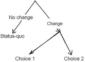
In the NL model, the scale factors or inclusive values (IVs) are related to the different level nodes. The IV is a measure of the attractiveness of a nest and corresponds to the expected value individual i obtains from alternatives within nest k. The IV parameters have values between 0 (perfect correlation) and 1 (no correlation or degree of similarity in the stochastic component of utility within each nest) if the NL is the correct model specification. When the IV parameter equals 1, the NL model is equivalent to the CL model (Train, 2003; Swait, 2007).

7.4.3 Covariance Heterogeneity Model

The Cov-Het model extends the NL model by parameterizing the scale factor (μ) with individual sociodemographic variables, rather than imposing the restriction that μ = 1. Models of scale heterogeneity essentially capture differences in respondent coherence, decision-making ability, and interest in the issue (Breffle and Morey, 2000). This contrasts with preference heterogeneity models, which analyze how the effect of choice attributes differ across individuals with different socioeconomic characteristics of individuals (Kontoleon, 2003). Whether individual characteristics should enter the model in terms of the scale parameter, rather than influencing tastes (e.g. through interactions with CE attributes), is a contentious point (Boxall and Adamowicz, 2002). However, it is clear that the scale issue needs to be addressed more fully to improve the estimates of preference part-worths and to provide a better understanding of the effects associated with different individuals’ levels of uncertainty.

7.4.4 Heteroscedastic Extreme Value Model

The HEV model is similar to a MNL or CL model, but it allows for heteroscedasticity in the utility function. The stochastic utility terms are independent Gumbel (Type 1 extreme value), but have different alternative-specific scale parameters μ (i.e. it has a different variance for each alternative). An HEV model can be used to assess any status quo effect and uncertainty in choices between alternatives. Swait and Adamowicz (1999) note that complexity of choice is reflected in the propensity to ‘avoid’ choice by deferring to the status quo and that because of complexity over choice contexts, preferences are characterized by different levels of variance. The HEV model relaxes the CL model assumption of equal variance for each alternative in the choice set. The HEV model is expressed as:

(7.4)

where μ_j denotes the different scale parameters across alternatives. The HEV model avoids the problem of any failure to meet the IID condition that is implicit in the CL model, by allowing different scale parameters across alternatives (Bhat, 1995). The random error term represents unobserved attributes of an alternative; in other words, the uncertainty associated with the expected utility (or the observed part of utility) of an alternative. The larger the scale parameter of the random component for an alternative and, conversely, the smaller the variance, the more tempered is the effect of a change in observed utility differential (Louviere et al., 2000).

HEV models have been used to investigate preferences for the attributes of an archaeological site in terms of the status quo, and choice uncertainty and variance associated with alternative attribute bundles (Willis, 2009). Visitors to archaeological sites typically exhibit little uncertainty associated with the current situation or status quo alternative, but exhibit much more uncertainty or variance, ceteris paribus, with alternative and hypothetical attribute packages that would change the characteristics of an archaeological site.

7.4.5 Mixed Logit and Random Parameter Logit Models

The panel MXL model was developed to account for the intuitive fact that decision agents differ from each other. The common formulation is that they differ in terms of taste intensity (Train, 1998), leading to the following utility specification:

(7.5)

The utility function of each consumer has some random taste parameters with values that depend on the values of the parameters θ of an underlying distribution . Thus the RPL includes heterogeneity of preferences through the systematic component of utility ′x_ij.

The choice of distribution strongly affects the properties of the model (Hensher and Greene, 2003). Such random taste parameters induce correlation across choices made by the same agent but maintain the advantageous logit probability. In fact, ɛ_ij is an IID Gumbel and hence, conditional on the parameter draw, the choice probability is still logit. In the RPL model the researcher has to decide on the parameterization of the covariance matrix (i.e. whether preference parameters are assumed to be independent or correlated).

Functional forms for the taste distributions include normal, log-normal, uniform, and triangular. The log-normal distribution is useful if the coefficient is known to have the same sign for each decision maker, which explains its use to estimate the price coefficient.⁵ The uniform distribution with a (0, 1) bound is suitable for dummy variables (Hensher and Greene, 2003, p. 145). However, the log-normal distribution typically has a long right-hand tail, so the use of the log-normal distribution for the price coefficient can lead to a low coefficient value for price and consequently a high WTP value for a unit change in an attribute. This explains why the price coefficient is often fixed in a MXL model, even though normal or log-normal distributions are assumed for other attributes. The uniform and triangular distributions have the advantage of being limited between the values ‘b − s’ and ‘b + s’, where the mean b and spread s are parameters to be estimated (Hensher and Green, 2003). Colombino and Nese (2009) experimented with normal, uniform, and triangular distributions in estimating policies for management of the archaeological site at Paestum in Italy; attributes included opening times, audio guides, guided tours, café, exhibitions, events, laboratory, audiovisual, documentation center, and price of admission. Paestum, originally founded as a Greek city before being taken over by the Romans in 273 BC, is exceptionally well preserved, with three imposing Greek Doric temples: Hera (550 BC), Ceres (originally dedicated to Athena 500 BC), and Neptune (originally dedicated to Poseidon 450 BC). Colombino and Nese (2009) found that the attribute coefficients were similar whether a normal, uniform, or triangular distribution was adopted. They also found a lower interest (negative WTP) for the development of a café on site, but that visitor preferences were heterogeneous across attributes with, for example, 46% of respondents having a positive utility for a café.

MXL was used by Jaffry and Apostolakis (2011) to investigate preferences and WTP amongst visitors to the British Museum in London for future management initiatives relating to attributes including opening hours, specialist exhibitions, staffing levels, facilities, information about museum exhibits, and community engagement. They found a MXL model provided better predictions of individual choice patterns than a CL model. Both visitors and non-visitors to the museum preferred more specialist temporary exhibitions throughout the year and greater provision of information. Temporary specialist exhibitions provide a greater incentive to visit a museum and also act as a pulling factor for the permanent exhibitions at the museum. CEs are most successful in estimating values and preferences for the contents of museums and art galleries when respondents have clear preferences (either for or against) particular sections of museums or exhibits. For various reasons this may not be the case for some art museums (Kinghorn and Willis, 2007), although visitors usually have clear preferences when visiting museums that have received considerable media attention such as the Tate Modern in London.

The marginal choice probabilities in a MXL model are obtained by integrating the distribution density over the range of parameter values:

(7.6)

Breffle and Morey (2000) are amongst the few who investigated heterogeneity in scale. In their model it is the scale of the Gumbel error rather than taste intensity that varies randomly across respondents, so that the utility function is:

(7.7)

This explicitly accounts for the fact that the same taste intensities might be associated with more or less utility variance (inversely related to error scale) in different choice agents. This may be due, for example, to differences across individuals or households in the evaluation of utility associated with different cultural goods.

A RPL model was used by Morey and Rossmann (2003) to investigate people’s preferences and WTP for the preservation of 100 major marble monuments in Washington, DC that were exposed to air pollutants such as sulfur dioxide. A normal distribution was specified for each random preference parameter. A normal distribution implies that, for any increase in preservation, a proportion of the population will consider it a bad (i.e. have a negative compensating variation).⁶ The Morey and Rossmann model also included the socioeconomic characteristics of respondents. They found WTP to preserve the monuments varied significantly across individuals. For most individuals WTP was positive and significant, but negative for a significant proportion of young non-Caucasians.

MXL models often provide a much better fit to the data than CL models, allowing for the panel structure of the data and correlation across choices (i.e. correlation in the error terms common to responses of a given respondent). Using a MXL model, Willis and Snowball (2009) revealed heterogeneity of taste in people attending theater shows of the National Arts Festival in South Africa. There was considerable heterogeneity of taste with respect to whether the cast was ‘professional’, whether the play was a ‘classic’, and for shows classified as ‘drama’.

The estimated mean and standard deviation of the attribute coefficients in MXL models provide information on the share of respondents who have positive and negative utilities for each attribute in the model. Thus, Willis and Snowball (2009) used a normal distribution for tastes around each attribute, and derived a coefficient for shows with professional casts of 0.57014 and a coefficient for the standard deviation of 0.74807. The normal distribution implies that 78% of the distribution is above zero and 22% below, suggesting that a production with a professional cast is an inducement to 78% of theater-goers and a negative factor for 22%, who apparently prefer amateur casts. In terms of type of show, drama appealed in varying degrees to 87% of theater-goers, but was unappealing to 13% of patrons.

The MXL model can also be used to explore individual preferences for theatrical productions. Individual-based parameters are interesting in that they provide precise information of individual tastes in the sample, and identify the degree of heterogeneity in tastes and preferences. Individual-specific parameters are also useful for management and marketing purposes, in pricing and in the selection of artistic productions to stage, since they provide information on the distribution of tastes and WTP. Individual-specific parameters can also be applied to derive consumer surplus estimates and the social valuation of cultural goods.

Individual parameters can be obtained from the MXL model conditioning the population distribution of parameters β, either on the real choices made by the individual (Grisolia and Willis, 2011b) or on the consumer market segment to which the individual belongs if RP data are not available (Scarpa et al., 2004). This information works as a prior in Bayes’ rule. Considering individual choices Y_n it is possible to derive the conditional density h(β_n|y_n) of any β_n taking the Bayes’ rule:

(7.8)

This ratio shows that the conditional distribution (hβ_n|y_n) of the individual parameters can be obtained as the probability of observing the individual choices given β_n multiplied by all range of betas in the population, divided by the probability of observing these choices in the population of betas (Train, 2003; Grisolia and Willis, 2011a).

7.4.6 Error Components Models

In an EC model utility is specified as:

(7.9)

where x_ij and z_ij are vectors of observable variables related to alternative j, α is a vector of fixed coefficients, ψ is a vector of random terms with zero mean, and ɛ_ij are IID (Train, 2003). Unlike a RPL or MXL model, coefficients are fixed, but the ECs allow for correlations between alternative choice bundles. The additional EC can be either independent across choices (e.g. in a non-panel structure Cov(ψ_nj,ψ_ni)) or it can be the same for all choices made by the same individuals (in a panel implementation). This is relevant in CEs as it breaks away from the assumption of independence in the error structure across choices by the same respondents which is implicit in both conditional and NL assumptions. The EC, shared across choice occasions, can be captured by an EC model and this allows for greater heterogeneity in individual preferences. The importance of all this remains an empirical issue to be investigated on a case-by-case basis. However, within the same category of model and estimation procedure, it can be assessed on the basis of log-likelihood values. For this reason both non-panel and panel EC models are often estimated (Scarpa et al., 2005, 2007).

The ECs ψ_nj might be associated with a hypothetical choice compared to the status quo. The reason is that while the status quo alternative is familiar to the respondent and hence prone to a smaller individual valuation error, the alternatives associated with change are hypothetical in nature and hence a larger fraction of their stochastic component is likely to be subject to unobservable error. Thus, the EC model is analogous to the NL and the HEV models in addressing the IIA issues, and allowing a more flexible substitution pattern between alternatives. An EC model with socioeconomic categories can reveal how the variance–covariance structure of unobservable components varies by category of consumer.

7.4.7 Multinomial Probit Model

The MNP model is a flexible model – it allows random taste variation, can represent any substitution pattern, and is applicable to panel data with correlated errors. It therefore avoids the restrictive substitution patterns in the IIA assumption.

The MNP model is:

(7.10)

where β_i ∼ N(b,Σ_β), ɛ_i = (ɛ_i1,…, ɛ_iJ)′ ∼ N(0,Σ_ɛ). Thus, the MNP model assumes a normal distribution for all unobserved components of utility. This might be a reasonable assumption for most attributes, but is problematic for price since a normal distribution with a density on both sides of zero implies some people have positive price coefficients. If the particular cultural good is a positional good, or a Veblen good, where demand increases as price increases, then a MNP model might be applicable.

Swait (2007) showed the commonality of many CE models, with the MNP model mimicking the MNL when the covariance matrix has the same variance for all alternatives, and mimicking the HEV model if variances are alternative-specific. Dahlberg and Eklöf (2003), in an analysis of Tiebout migration (destination choices in response to variations in the quality of local public services, including cultural services), derived similar values for the compensating variation from CL, MXL, and MNP models.

7.4.8 Latent Class or Finite Mixture Models

In the MXL model the mixing distribution f(β) or density function is continuous over the specified function; β may be specified, for example, to be normal with mean b and covariance W. However, if the mixing distribution f(β) has a fixed set of finite values within a group or population class, the MXL model becomes a LC model. Each finite value corresponds to a segment of population, with each class having a distinct and different set of preferences, choice behavior, and attribute coefficients. Thus, heterogeneity is introduced in LC models by assuming the distribution of tastes and utility functions vary between ‘latent’ (i.e. as yet unobserved) classes or groups of individuals, whilst assuming preferences within each LC are homogeneous.

LC analysis has been used to explore homology, individualization and omnivore–univore arguments in cultural consumption (Chan and Goldthorpe, 2007). Part of the appeal of LC analysis is that labels or names can be attached to different segments of cultural consumption (e.g. ‘univore’, ‘omnivore’ or ‘high-brow’ and ‘low-brow’). Pulido-Fernández and Sánchez-Rivero (2010) used a LC approach to analyze cultural tourism in Andalusia, Spain, and identified ‘museum culturophiles’, ‘culturally inactive’, and ‘roaming culturophiles’. LC models have also been used to analyze consumption preferences and heterogeneity of taste in recreation and cultural choices. Boter et al. (2005) identified four museum market segments in the Netherlands from visitor patterns: large art museums, regional museums, large museums in the Randstad (i.e. the four largest Dutch cities and the surrounding areas) with varied collections, and museums in peripheral regions of the Netherlands with a variety of collections. The segments differed in terms of attributes such as willingness to travel, percentage of youth-card holders visits, and type of collection visited. Boter et al. found willingness to travel to regional museums was only half as large as that for large art museums.

Scarpa and Thiene (2005) used a LC approach to investigate ‘lumpy preferences’ of a sample of rock climbers. The sample covered day trips to six areas in the ‘pre-Alps’ in the Italian Alps and 12 areas in the Dolomites proper. Variables distinguishing the LCs were travel cost, access, severity, difficulty of climb, climbers’ characteristics, number of climbs, and Alp location. Colombo et al. (2009) found a LC model to be superior to both a RPL and a HEV model in assessing preferences and WTP for cultural heritage landscapes in upland areas of England. The attributes comprised changes in heather moorland and bog, rough grassland, mixed and broadleaved woodlands, field boundaries (stone walls), traditional farm buildings and practices, and tax payment. Preference heterogeneity was better explained in terms of LCs than at an individual level in terms of deterministic utility; in this case, heterogeneity was better captured in the systematic utility component rather than the random component.

Grisolia and Willis (2012) used a LC model to identify three classes of theater-goer at a regional theater in England, with their respective market shares. The largest and ‘main class’ comprised mainly affluent people with a strong preference for the main theater venue, who considered reviews of the productions and whether the author was known, and who liked all types of shows. The second, a ‘popular class’, exhibited the smallest WTP and had a strong preference for comedies, paid little attention to venue, and disliked more sophisticated shows. The third, an ‘intellectual class’ of theater-goer, exhibited the highest WTP, and had a strong interest in drama and adaptation of productions, and exhibited more independent aesthetic judgment.

An important aspect of LC analysis is determining the number of segments or LCs. One procedure is to compare the adjusted pseudo-R² statistic as the number of LCs is increased sequentially (S = 1, 2, 3,…). If the pseudo-R² increases with more LCs, this indicates the presence of heterogeneity in the choice data. When additional LCs do not increase the pseudo-R² statistic, the number of LCs is determined. Alternatively, the AIC (Akaike Information Criterion) or BIC (Bayesian Information Criterion) statistics can be used and a decision based on the model with the lowest AIC or BIC criterion, since the lower the AIC or BIC statistic, the better the fit of the model. Provencher et al.,2002 discuss the relative merits of AIC and BIC in determining the number of LCs. If the information criterion does not unambiguously determine the number of LCs, then additional conditions could include judgments on the conformity of coefficients and coefficient signs to theoretical expectations across the LCs.

7.5.1 Measures of Economic Welfare

The coefficients in discrete CE provide estimates of the utility of each attribute. In CEs the price coefficient is interpreted as an estimate of the negative marginal utility of income. In the CL or MNL model, the marginal value of an attribute is the ratio of the coefficient of an attribute to the coefficient of price: MWTP = −α₁/β_p, where α₁ is the coefficient for attribute 1 and β_p is the coefficient for price. This is an ‘implicit price’ that represents WTP for a unit change in the quantity of an attribute, in whatever units the attribute is defined in the CE. If a quadratic term is specified for an attribute, the MWTP depends upon the scale of the change in the attribute level. This approach of deriving implicit prices by calculating the ratio of non-cost parameters to the cost parameter can lead to unreasonably high estimates of implicit prices if the cost parameter is close to zero.

In MXL models, if the attribute has been specified to have a log-normal rather than a normal distribution, the log of the coefficients is distributed normal with mean m and standard deviation s, and the coefficients themselves have mean exp(m + (s²/2) with a standard deviation equal to the mean times √((exp(s²) − 1) (Train, 2003, p. 275). In MXL models, the mixing distribution for price is either specified as a log-normal (to avoid positive price coefficients) or it is assumed to be fixed. However, a fixed cost parameter implies the marginal utility of money is homogeneous across all respondents and also that the scale parameter is the same across all observations (Hensher and Greene, 2011).

Different forms of welfare measure can be calculated from CE model information. Compensating variation can be calculated, namely the amount of money that can be taken away from (or returned to) a household after a specified improvement (decrement) in cultural heritage and still leave the household at its original utility position (the status quo utility position). The change in cost of cultural heritage that would result in X% of households consuming a particular cultural heritage good can also be calculated. If gains and losses of a cultural good have been included in the experimental design, then asymmetry in value between gains and losses can be estimated. Asymmetry can be estimated in different ways: by specifying a non-linear function, calculating separate coefficients for increases and decreases in price, and estimating a fixed effects model with dummy variables for gains and losses in the levels of the good (Lanz et al., 2010).

Different CE models (MNL, NL, HEV, MXL-RP, EC, and MNP) can produce different estimates of WTP for the same attribute. In a valuation study of the use of the Old Parliament House in Canberra, which is now a museum, Choi (2009) examined the stability of WTP for the frequency of temporary exhibitions in the museum using a MNL and three MXL models, each of which had slightly different variables and different treatments of the alternative specific constant (ASC).⁷ He also varied the coding of facilities (shop, café, and fine dining) as dummy or effect coded.⁸ He found differences in WTP estimates for temporary exhibitions across the four models with those derived from the MNL and MXL, with an ASC being much higher than those derived from the two MXL models in which the museum facilities were dummy and effect coded. This clearly points to the importance of selecting the best model to fit the data, the model which appropriately accounts for the relative heterogeneity between the systematic components and the random error component of utility, and the model which has an appropriate functional form (linear or non-linear variables), if the most accurate, reliable, and robust estimate of WTP for an attribute is to be obtained.

7.5.2 Willingness to Pay Re-Parameterization

The utility specifications discussed so far are all in preference space, but most economic investigations focus on WTP estimation. In such contexts a potentially more advantageous re-parameterization of utility is one in WTP space (Cameron and James, 1987; Train and Weeks, 2005; Sonnier et al., 2007). In panel MXL models these specifications can both account for scale variation and isolate utility coefficients that can immediately be interpreted as marginal WTP effects. If α_i is the cost coefficient, the WTP specification of utility takes the generic form of:

(7.11)

where w_i = β_i/−α_i is a vector of marginal WTP for each of the choice attributes. Without random taste or scale variation Eq. (7.11) is only a re-parameterization of Eq. (7.2). However, the results may be more convenient because coefficient estimates are interpretable in the money space and so are the estimated standard errors; the latter no longer need to be derived using simulation (Poe et al., 2005) or closed-form approximations obtained, for example, via the delta method (Goldberger, 1991).

In panel MXL this specification has the advantage of allowing the researcher to exercise a better control over the distribution of marginal WTP values in the population. These values are otherwise jointly determined by the distributional assumptions for the attribute and money coefficients, which give, respectively, the numerator and denominator of individual WTP estimates (Scarpa et al., 2008). Values can be estimated directly in WTP space using BIOGEME (Bierlaire, 2003).

7.5.3 Market Share

In CV total WTP or demand is derived by multiplying the number of consumers who are willing to pay a specific price, by that price, and summing across all price levels. Similarly in CEs it is important that total WTP is only based on that segment of the population, or market share, who are willing to pay for an improvement to the status quo level. If k is the status quo and j the new cultural heritage level, then is the odds ratio of the probability of choosing alternative j over the baseline k when cultural heritage is changed from x_ik to . Such an analysis indicates how public acceptability of cultural heritage would change from the status quo if a particular policy were implemented. This change in the odds ratio, or the odds of choosing one alternative over another, is a feature of respondents’ preferences for one level of cultural heritage over another, and the public acceptability or market for a change in cultural heritage provision.

The ‘true’ effect on welfare of a change in cultural heritage provision is measured by the amount of money (Δ$) households are willing to pay for a positive change or are willing to accept for a negative change. This is the amount that sets the two utility levels equal to each other. The general formula is:

(7.12)

where β_i is the parameter estimate for the attribute i, x is the numerical level for a particular cultural attribute, α is the parameter estimate for the utility of money, the superscripts 0 and 1 refer, respectively, to the initial and final state, and the subscript i refers to the generic ith attribute. Thus, a change in value is given by the sum of the products between part-worths of each cultural attribute and the respective change in provision Δx_i (Willis, 2006).

7.6.1 Interaction Effects Between Attributes

In an experimental design, main effects indicate the change produced by varying one factor or attribute averaged over all levels of the remaining factors. A two-factor interaction, A × B, reveals whether, averaged over all levels of the remaining factors, the effect of varying A is the same for all levels of B. A three-factor interaction, A × B × C, shows whether, averaged over all levels of the remaining factors, the interaction between any two of A, B, C, say A and B, is the same for all levels of the third factor C. Main effects tend to be more important than two-factor interactions, which in turn are usually much more important than three-factor interactions. SP models, including CV methods, rarely consider interactions between factors. Santos (1998) revealed considerable interaction effects between the three principal attributes (stone walls and barns, flower-rich meadows, and small-farm woodland) of an upland heritage landscape that was subject to environmental policy and subsidies. Willis (2009) revealed interactions between some attributes in a CE of visitors’ preferences and tastes for the attributes of a Roman fort along Hadrian’s Wall, which once marked the boundary of the Roman Empire in northern England; the attributes included excavations, information displays, museum, replica reconstruction of some buildings, amenities (café, etc.), and proposed children’s play area.

Failure to account for interaction effects in CEs can result in a considerable overestimation or underestimation of the value of the good as a whole, when the total value is derived by summing the part-worths or the value of individual attributes. Failure to account for interaction effects is a failure to account for substitution effects between attributes. CEs may overestimate the value of a good compared to a CV estimate when only a main effect experimental design is used and the attributes are assumed to be linearly additive. Indeed, Mogas et al. (2006) noted that CE and CV were equivalent in valuing alternative afforestation programs in northeast Spain when more fully specified utility functions (specifically, second-order effects) were included. However, when elements of the utility functions (i.e. second-order interaction effects) were omitted, CE estimates were much higher than CV estimates.

7.6.2 Choice Complexity

Swait and Adamowicz (1999) theorized that consumers faced with increasing choice complexity might be less able to make ‘accurate’ choices and thus their preferences might be characterized by different levels of variance depending on the complexity of the task. They also hypothesized that complexity of choice is related to the propensity to ‘avoid’ choice by deferring choice or choosing the status quo. The effect of task complexity on variance was quantified in an empirical study by DeShazo and Fermo (2002). They investigated whether complexity in choice sets impacted on choice consistency and welfare estimates. An increase in the number of attributes was found to increase the variance of the EC in utility, suggesting that increased cognitive burden associated with greater information outweighed the potential increase in consistency induced by a more complete description of the product’s attributes. An increase in the number of alternatives was found to initially decrease error variance and then to increase it. They also found that increasing the number of attributes that differed across choice alternatives substantially increased the variance of utility.

Any bias in CE might be minimized through pre-testing the experimental design and questionnaire to control for choice complexity, to identify the optimal number of alternatives in choice sets, and to optimize the number of attributes that vary across choice alternatives.

7.6.3 Non-Attendance

Evidence suggests that individuals use heuristics when choices are complex to choose an alternative attribute bundle. This process can be investigated in different ways. (i) A check can be made to see if respondents make tradeoffs against price in the choice sets. The number who consistently chose the status quo across all choice sets can be reported – this percentage should be low if there are some attribute improvements for little or no price increase. It can also be observed whether respondents chose different alternatives, and did not always simply choose alternative 1 or alternative 2. The proportion of respondents who select choice alternatives with larger and larger price increases can also be checked – the proportion should decline as price increases. (ii) Diagnostic or supplementary questions can be included in the questionnaire to investigate how attributes were processed and why respondents responded in the way they did in choosing options. This provides a useful additional check, but is more applicable to CV questions where analysis of tradeoffs between attributes cannot be undertaken other than by observing a declining acceptance rate as price increases. (iii) An analytical model can be developed to reveal the extent to which respondents adopt a particular processing strategy (e.g. whether given attributes are ignored or subject to non-attendance in the CE). Recently, Campbell et al. (2012) have analyzed response latency (a measure of the cognitive effort invested by respondents in a self-administered online SP survey) in an attempt to disentangle preference, variance, and processing heterogeneity, and to explore whether response latency helps to explain these three types of heterogeneity.

Ignoring attributes in a CE implies non-compensatory behavior and is likely to give rise to unreliable estimates of the marginal WTP for an attribute. Scarpa et al. (2009) modeled attribute non-attendance using a LC model in a study of cultural landscape preservation and enhancement in Ireland. The attributes were mountain land, stone walls, farm tidiness, cultural heritage, and cost. The most attended attribute was mountain land (probability 0.943), the least non-monetary attribute attended to was farmyard tidiness, but the attribute with the lowest probability of attendance (0.0865) was price. The probability of membership of a class in which all attributes were attended was 0.0566, although the probability of membership in a class where all attributes were ignored was only 0.0512. Thus, full weighted tradeoffs between attributes seems to be only applicable in a minority of cases. The probability of considering and valuing all attributes was less than 0.1 in the Ireland cultural landscape study (Scarpa et al., 2009). Most respondents seemed to ignore at least two of the five attributes and the cost attribute was often one element of the pair. As Scarpa et al. (2009) note, ‘if people chose alternatives as if cost was of little or no consequence, they behave as if they had a marginal utility of income of zero or close to zero’. Therefore WTP estimates using a standard CL or MNL model can be large where respondents ignore price and hence have a price coefficient close to zero. This induces a much higher WTP value for attributes, compared with a model accounting for attribute non-attendance. The failure to account for heterogeneity in processing heuristics in CEs will probably result in an overestimate of marginal WTP for specific attributes. What is of particular concern is the large failure to account for non-attendance with respect to cost, which may partly explain why CEs typically overestimate marginal WTP for environmental and cultural goods compared to CV methods (Scarpa and Willis, 2006).

7.6.4 Scale Versus Taste Heterogeneity

Utility has no units, so it is necessary to normalize its scale, typically defined by the variance of the error term in CE models. However, this variance can differ between datasets depending on their characteristics, meaning that parameters cannot be directly compared across diverse datasets except in the unlikely event that each dataset has the same variance. Isolating scale effects should result in better estimates of preference coefficients.

Standard choice modeling estimates the product μ_iβ rather than β. The scale parameter μ_i relates to the amount of certainty in respondent i’s expected choices. Differences in scale parameters are required to isolate meaningful comparisons of preferences or β parameters across individuals or groups. Response variance is inversely related to μ, with response variance being a measure of uncertainty. For individuals with μ approaching 0, the response variance approaches infinity which reflects complete uncertainty, in which case choice probabilities derived from the MNL model are equal for all alternatives (Magidson and Vermunt, 2007).

The scale parameter confound is assumed not to exist in CL models under the restrictive assumption that the level of uncertainty implied by the values of the scale parameter, is identical for each respondent. In CL and other conventional logit models such as LC models, the scale factor (μ) is normalized to unity for all respondents. However, if there are two subgroups (e.g. latent classes X and Y), whose true preferences for two goods are identical (e.g. +0.5 and +0.5 for good A, and +0.4 and +0.4 for good B), but who exhibit different degrees of uncertainty about these goods such that the scale parameter for group X = 1 and for group Y = 2, then the model coefficients for the two goods will be 0.5 and 0.4 for group X, but 1.0 and 0.8 for group Y. Yet the only true difference between the two groups of respondents is that responses obtained from the former group reflect greater amounts of uncertainty (Magidson and Vermunt, 2007).

Louviere et al. (2008) argued that much of the taste heterogeneity in choice is better described as ‘scale’ heterogeneity (i.e. the scale of the error term is greater for some consumers than for others). Fiebig et al. (2010) point out that the scale of standard error of the idiosyncratic error is not identified in DC data – a problem that is resolved by normalizing it to a constant. Fiebig et al. (2010) extend the MXL model to a ‘generalized MNL’ (G-MNL) model to assess whether including scale heterogeneity leads to a significant improvement in fit compared to a conventional MXL model. They found, for data from 10 different SP CEs covering different goods (medical procedures, mobile phones, food delivery services, holiday packages, and charge cards), that models including scale heterogeneity had a better goodness-of-fit than MXL models. Their G-MNL model was better able to account for extreme consumers who exhibit nearly lexicographic preferences and also for customers who exhibit very low ‘random’ behavior, compared to a MXL model.

No confound occurs in latent class choice models under the assumption that the values of the scale factor are the same for all respondents regardless of the latent class to which they belong (Louviere et al., 2000, p. 206). If the equality assumption is violated, the predictions contain additional amounts of error as well as potential bias. Magidson and Vermunt (2007) propose extended LC choice models that can be used to test the equal scale factor assumption, and when violated, to estimate and remove the effects of the different scale parameters that exist for different respondent subgroups. Isolating the scale factors should result in more pure measures of part-worth preference coefficients (i.e. true preferences for the different LCs based on part-worth preference utilities free from scale effects). Magidson and Vermunt (2007) argue that by not allowing differences in the scale factor to be a determinant in the formation of different LCs, the LC groups will more clearly differentiate respondents based on their ‘true’ preference differences based on scale-free part-worth utilities. Isolation of the scale factors will result in more accurate measures of ‘true’ part-worth utilities.

Applications of these new extended models in two real-world CEs find that in both cases the commonly made assumption of equal scale factors is unwarranted. Comparing results from the standard models with those from the extended models suggests that the former leads to some faulty conclusions regarding the actual part-worths, as well as misclassification of a substantial number of respondents into the wrong LC segment. The results also suggest that discrete-factor choice models, with and without a scale-factor adjustment, may well provide additional improvements both in data fit and in interpretation of results over the more traditional LC choice models.

7.6.5 WTP Versus WTA Asymmetry

The loss of a cultural good may be valued more highly than an equivalent gain in the good. This asymmetry between WTA compensation for the loss of a good and WTP for a gain has long been a feature of most CV results. Explanations for WTP–WTA asymmetry in terms of economic theory have emphasized the role of substitution and income effects (Hanemann, 1991, 1999). Disposable income constrains demand for cultural heritage in terms of WTP, but not WTA compensation. Moreover the unique character (low substitutability) of a good implies high compensation to offset utility loss. An alternative explanation for WTP–WTA asymmetry is ‘loss aversion’ (Kahneman and Tversky, 1979; Tversky and Kahneman, 1991), which is argued to be a superior predictor of economic behavior (Bateman et al., 1997). Loss-averse decision makers perceive losses as larger than equivalent physical gains in terms of utility. However, Plott and Zeiler (2005), using a BDM auction mechanism and subject training, found no difference between WTP and WTA across a variety of goods, thus calling into question loss-aversion theory in real-market conditions.

Lanz et al. (2010) found evidence of non-linearity in the underlying utility function even though the range of attribute levels was relatively small, revealing the presence of significant loss aversion in all attributes, including price. They also found coefficient estimates associated with losses to be of greater magnitude than those for gains and a tendency for the standard deviation coefficient to be greater for losses than for gains, implying greater heterogeneity in preferences for losses. In addition they found the WTP–WTA schedule to be asymmetric around the current provision level, but that the WTP–WTA ratio varied according to the particular good change under consideration. A linear model was also noted to provide a conservative estimate of WTA in comparison to the better-fitting non-linear models. However, different non-linear models produced substantially different WTA estimates, in spite of relatively small differences across models in terms of goodness-of-fit measures (Lanz et al., 2010).

7.6.6 Utility Maximization Versus Regret Minimization

Conventional CL, MXL, and other models assume that respondents, in selecting an alternative in a choice set, maximize utility. Respondents may be either consumers or decision makers conserving a cultural heritage good. There is some empirical evidence to suggest that regret minimization is a more important determinant of choice than utility maximization, especially where choices are difficult and important, and where decision makers may be held accountable for their choice. In one study Chorus et al. (2011) found that a random regret minimization (RRM) approach slightly outperformed a random utility maximization (RUM) approach. However, in an application to recreational site choice, Boeri et al. (2012) found the opposite – a RUM specification performed slightly better than a RRM approach, although for less familiar sites choice was better described by RRM. However, the two approaches (RUM and RRM) lead to different behavioral insights and can lead to different policy implications in terms of which cultural heritage goods to conserve.

7.6.7 Independent Valuation and Summation

Where there are many attributes, more than one CE is often used to value a good. This can give rise to the independent valuation and summation (IVS) problem (Hoehn and Randall, 1989). Various studies have shown, both in theory and practice, that an IVS approach grossly overestimates aggregate WTP when valuing goods independently where there are significant substitution effects. Additive separability⁹ is a common assumption in aggregating the values for different goods in space and time. However, where there are substitution effects between goods, additive separability or IVS cannot be applied. In an appraisal of three alternative programs, Hoehn and Loomis (1993) showed that conventional IVS estimates that valued each program separately overestimated the value of a two-program agenda by 12–50%, whilst the value of a three-program agenda was overestimated by 43–66%.

7.6.8 Attitudes

Substantial efforts have been made to incorporate heterogeneity into DC models by including socioeconomic characteristics of the individual, and through random variation in systematic and random components of the model. More attention needs to be given to the inclusion of behavioral and psychological factors in determining choice in DC models. Following the work of Ajzen (1988) and Domarchi et al. (2008), Scagnolari and Maggi (2010) constructed indicator scores to assess young people’s attitudes towards alcohol consumption, social norms, and perceived behavioral control. They used these indicators to assess choice of night-time entertainment (dinner, after-dinner venue, and size of group). Psychological characteristics were found to have more influence on leisure night-time activity choices than hard information on socioeconomic characteristics. They found that different night-time activities can be explained by alcohol consumption attitudes, and that the inclusion of behavioral and psychological characteristics greatly enhanced DC model realism and goodness-of-fit of the model.

7.6.9 Combined Revealed Preference and Stated Preference Model

SP experiments can be combined with RP data where additional information is required about changes in preferences and behavior from the introduction of a new attribute. This is not a recent phenomenon, but it brings us full circle to where we started the chapter (i.e. the relative merits of using RP or an SP approach). Including RP with SP data does allow estimates to be based on what people do, as well as on what they say they would do.

Boxall et al. (2003) included a SP experiment in which canoeists to wilderness canoe routes in Manitoba, Canada were asked if they would change their route choices in response to the presence of ‘pristine’ and ‘spoilt’ 2000-year-old aboriginal rock paintings. This experiment produced pooled RP and SP information for the same set of individuals. Consistency between the RP and SP datasets was judged in terms of the scale parameter. Whilst the scale parameter (μ) is not identifiable in one dataset, their ratios (μ_rp/μ_sp) can be identified in two or more datasets. Pooling assumes statistical independence of revealed and SPs from the same individual. Boxall et al. (2003) allowed for this in their RP/SP data by accounting for potential dependence or correlation between RP and SP choices. The SP data indicated that 42% of respondents would change their route to another to view a pristine painting, but only about 10% would do so to see a defaced painting. WTP to view pristine paintings added about $77 to the value of the trip, but defaced paintings were only worth about 10% of the value of pristine paintings. The authors concluded that the greater value of pristine paintings over defaced paintings pointed to the need to control vandalism to cultural sites, in order to preserve heritage for the benefit of future visitors.

References

1. Ajzen I. Attitudes, Personality and Behaviour. Milton Keynes: Open University Press; 1988.
2. Alberini A, Longo A. Combining the travel cost and contingent behaviour methods to value cultural heritage sites: evidence from Armenia. Journal of Cultural Economics. 2006;30:287–304.
3. Bateman IJ, Munro A, Rhodes B, Starmer C, Sugden R. A test of the theory of reference-dependent preferences. Quarterly Journal of Economics. 1997;112:479–505.
4. Bateman IJ, Langford IH, Jones AP, Kerr GN. Bound and path effects in double and triple bounded dichotomous choice contingent valuation. Resource and Energy Economics. 2001;23:191–213.
5. Bhat C. A heteroscedastic extreme value model of intercity mode choice. Transportation Research B. 1995;29:471–483.
6. Bierlaire, M., 2003. BIOGEME: a free package for the estimation of discrete choice models. Paper Presented at the 3rd Swiss Transport Research Conference, Ascona.
7. Boeri M, Doherty E, Longo A, Hynes S. Site choices in recreation demand: a matter of utility maximization or regret minimization? Journal of Environmental Economics and Policy. 2012;1:32–47.
8. Boter J, Rouwendal J, Wedel M. Employing travel time to compare the value of competing cultural organizations. Journal of Cultural Economics. 2005;29:19–33.
9. Boxall PC, Adamowicz WL. Understanding heterogeneous preferences in random utility models: a latent class approach. Environmental and Resource Economics. 2002;23:421–446.
10. Boxall PC, Englin J, Adamowicz WL. Valuing aboriginal artifacts: a combined revealed-stated preference approach. Journal of Environmental Economics and Management. 2003;45:213–230.
11. Breffle WS, Morey ER. Investigating preference heterogeneity in a repeated discrete-choice recreation demand model of Atlantic salmon fishing. Marine Resource Economics. 2000;15:1–20.
12. Cameron T, James M. Efficient estimation methods for closed-ended contingent valuation survey data. Review of Economics and Statistics. 1987;69:269–276.
13. Campbell, D., Morkbak, M.R., Olsen, S.B., 2012. Response latency in stated choice experiments: impact on preference, variance and processing heterogeneity. Paper Presented to the Annual European Association of Environmental and Resource Economists, Prague.
14. Carson RT, Mitchell RC, Conaway MB. Economic benefits to foreigners visiting Morocco accruing from the rehabilitation of the Fes Medina. In: Navrud S, Ready RC, eds. Valuing Cultural Heritage: Applying Environmental Valuation Techniques to Historic Buildings. Cheltenham: Edward Elgar; 2002;118–141.
15. Carson RT, Groves T. Incentive and informational priorities of preference questions. Environmental and Resource Economics. 2007;37:181–210.
16. Chan TW, Goldthorpe JH. Social stratification and cultural consumption: music in England. European Sociological Review. 2007;23:1–19.
17. Chilton S, Jones-Lee M, McDonald R, Metcalfe H. Does the WTA/WTP ratio diminish as the severity of a health complaint is reduced? Testing for smoothness of the underlying utility of wealth function. Journal of Risk and Uncertainty. 2012;45:1–24.
18. Choi AS. Willingness to pay: how stable are the estimates? Journal of Cultural Economics. 2009;33:301–310.
19. Chorus CG, Annema JA, Mouter N, van Wee B. Modeling politicians’ preferences for road pricing policies: a regret-based and utilitarian perspective. Transport Policy. 2011;18:856–861.
20. Colombino U, Nese A. Preference heterogeneity in relation to museum services. Tourism Economics. 2009;15:381–395.
21. Colombo S, Hanley N, Louviere J. Modeling preference heterogeneity in stated choice data: an analysis for public goods generated by agriculture. Agricultural Economics. 2009;40:307–322.
22. Cooper J, Loomis J. Sensitivity of willingness-to-pay estimates to bid design in dichotomous choice contingent valuation models. Land Economics. 1992;68:211–224.
23. Coursey DL, Hovis JL, Schulze WD. On the supposed disparity between willingness to accept and willingness to pay measures of value. Quarterly Journal of Economics. 1987;102:679–690.
24. Dahlberg, M., Eklöf, M., 2003. Relaxing the IIA assumption in locational choice models: a comparison between conditional logit, mixed logit, and multinomial probit models. Working Paper, Department of Economics, Uppsala University, Uppsala.
25. Davidson P, Teye-Ali C, Thomas A. Fundaments of discrete choice part 2 – the nested logit model. Traffic Engineering and Control. 2009;50:63–71.
26. Davis DD, Holt CA. Experimental Economics. Princeton, NJ: Princeton University Press; 1993.
27. DeShazo JR, Fermo G. Designing choice sets for stated preference methods: the effects of complexity on choice consistency. Journal of Environmental Economics and Management. 2002;44:123–143.
28. Domarchi C, Tudela A, Gonzalez A. Effect of attitudes, habit, and affective appraisal on mode choice: an application to university workers. Transportation. 2008;35:585–599.
29. Favaro D, Frateschi C. A discrete choice model of consumption of cultural goods: the case of music. Journal of Cultural Economics. 2007;31:205–234.
30. Ferrini S, Scarpa R. Designs with a priori information for nonmarket valuation with choice experiments: a Monte Carlo study. Journal of Environmental Economics and Management. 2007;53:342–363.
31. Fiebig DG, Keane MP, Louviere J, Wasi N. The generalized multinomial logit model: accounting for scale and coefficient heterogeneity. Marketing Science. 2010;29:393–421.
32. Foster, V., 1999. On the voluntary financing of public goods. PhD Thesis, Department of Economics, University College London.
33. Goldberger AS. A Course in Econometrics. Cambridge, MA: Harvard University Press; 1991.
34. Grisolia JM, Willis KG. An evening at the theatre: using choice experiments to model preferences for theatres and theatrical productions. Applied Economics. 2011a;43:3987–3998.
35. Grisolia JM, Willis KG. Heterogeneity in willingness-to-pay for theatre productions: individual specific willingness-to-pay estimates for theatres, shows and their attributes. Scottish Journal of Political Economy. 2011b;58:378–395.
36. Grisolia JM, Willis KG. A latent class model of theatre demand. Journal of Cultural Economics. 2012;36:113–139.
37. Gujarati D. Essentials of Econometrics. New York: McGraw-Hill; 1992.
38. Haab TC, McConnell KE. Referendum models and negative willingness to pay: alternative solutions. Journal of Environmental Economics and Management. 1997;32:251–270.
39. Hanemann WM. Welfare evaluations in contingent valuation experiments with discrete response data: reply. American Journal of Agricultural Economics. 1989;71:1057–1061.
40. Hanemann WM. Willingness to pay and willingness to accept: how much can they differ? American Economic Review. 1991;81:635–647.
41. Hanemann WM. The economic theory of WTP and WTA. In: Bateman IJ, Willis KG, eds. Valuing Environmental Preferences: Theory and Practice of the Contingent Valuation Method in the US. EU and Developing Countries: Oxford University Press, Oxford; 1999;43–93.
42. Hensher DA, Greene WH. The mixed logit model: the state of practice. Transportation. 2003;30:134–176.
43. Hensher DA, Greene WH. Valuation of travel time savings in WTP and preference space in the presence of taste and scale heterogeneity. Journal of Transport Economics and Policy. 2011;45:505–525.
44. Hoehn JP, Randall A. Too many proposals pass the benefit cost test. American Economic Review. 1989;79:544–551.
45. Hoehn JP, Loomis JB. Substitution effects in the valuation of multiple environmental programs. Journal of Environmental Economics and Management. 1993;25:56–75.
46. Jaffry S, Apostolakis A. Evaluating individual preferences for the British Museum. Journal of Cultural Economics. 2011;35:49–75.
47. Kahneman D, Tversky A. Prospect theory: an analysis of decision under risk. Econometrica. 1979;47:263–292.
48. Kinghorn N, Willis KG. Estimating visitor preferences for different art gallery layouts using a choice experiment. Museum Management and Curatorship. 2007;22:43–58.
49. Kinghorn N, Willis KG. Measuring museum visitor preferences towards opportunities for developing social capital: an application of a choice experiment to the Discovery Museum. International Journal of Heritage Studies. 2008;14:555–572.
50. Kontoleon, A., 2003. Accounting for consumer heterogeneity in preference for GM foods: an application of the latent market segmentation model. Paper Presented to the 4th BIOECON Workshop on the Economics and Biodiversity Conservation, Venice.
51. Kuhfeld WF. Experimental design, efficiency, coding, and choice designs. Cary, North Carolina: SAS Institute; 2005; TS-772C.
52. Lancaster KJ. A new approach to consumer theory. Journal of Political Economy. 1966;74:132–157.
53. Lanz B, Provins A, Bateman I, Scarpa R, Willis K, Ozdemiroglu E. Investigating willingness to pay – willingness to accept asymmetry in choice experiments. In: Hess S, Daly A, eds. Choice Modelling: The State-of-the-Art and the State-of-Practice: Proceedings from the Inaugural International Choice Modelling Conference. Bingley: Emerald Publishers; 2010;517–541.
54. Louviere JJ, Hensher DA, Swait JD. Stated Choice Methods: Analysis and Applications. Cambridge: Cambridge University Press; 2000.
55. Louviere JJ, Street D, Burgess L, Wasi N, Islam T, Marley AAJ. Modelling the choice of individual decision-makers by combining efficient choice experiment designs with extra preference information. Journal of Choice Modelling. 2008;1:128–163.
56. Luksetich WA, Partridge MD. Demand functions for museum services. Applied Economics. 1997;29:1553–1559.
57. Maddison D, Foster T. Valuing congestion costs in the British Museum. Oxford Economic Papers. 2003;55:173–190.
58. Magidson, J., Vermunt, J.K., 2007. Removing the scale factor confound in multinomial logit choice models to obtain better estimates of preference. In: Proceedings of the Sawtooth Software Conference, Santa Rosa, CA, pp. 139–154.
59. McFadden D. Conditional logit analysis of qualitative choice behavior. In: Zarembka P, ed. Frontiers in Econometrics. New York: Academic Press; 1973;105–142.
60. Mitchell R, Carson R. Using Surveys to Value Public Goods: The Contingent Valuation Method. Washington, DC: Resources for the Future; 1989.
61. Morey E, Rossmann KG. Using stated preference questions to investigate variations in willingness to pay for preserving marble monuments: classic heterogeneity, random parameters, and mixture models. Journal of Cultural Economics. 2003;27:215–229.
62. Mogas J, Riera P, Bennett J. A comparison of contingent valuation and choice modelling with second-order interactions. Journal of Forest Economics. 2006;12:5–30.
63. Mourato S, Kontoleon A, Danchev A. Preserving cultural heritage in transition economics: a contingent valuation study of Bulgarian monasteries. In: Navrud S, Ready RC, eds. Valuing Cultural Heritage: Applying Environmental Valuation Techniques to Historic Buildings, Monuments and Artifacts. Cheltenham: Edward Elgar; 2002;68–86.
64. Narwold A. Estimating the value of the historical designation externality. International Journal of Housing Markets and Analysis. 2008;1:288–295.
65. Neill HR, Cumming RG, Ganderton PT, Harrison GW, McGuckin T. Hypothetical surveys and real economic commitments. Land Economics. 1994;70:145–154.
66. Noonan DS. Contingent valuation and cultural resources: a meta-analytic review of the literature. Journal of Cultural Economics. 2003;27:159–176.
67. Oczkowski E. A hedonic price function for Australian premium table wine. Australian Journal of Agricultural Economics. 1994;38:93–110.
68. Plott CR, Zeiler K. The willingness to pay/willingness to accept gap, the endowment effect, subject misconceptions and experimental procedures for eliciting valuations. The American Economic Review. 2005;95:530–545.
69. Poe GL, Giraud KL, Loomis JB. Computational methods for measuring the difference of empirical distributions. American Journal of Agricultural Economics. 2005;87:353–365.
70. Powe NA, Garrod GD, Willis KG. Valuation of urban amenities using a hedonic price model. Journal of Property Research. 1995;12:137–147.
71. Provencher B, Baerenklau KA, Bishop RC. A finite mixture logit model of recreational angling with serially correlated random utility. American Journal of Agricultural Economics. 2002;84:1066–1075.
72. Pulido-Fernández JI, Sánchez-Rivero M. Attitudes of the cultural tourist: a latent segmentation approach. Journal of Cultural Economics. 2010;34:111–129.
73. Rolfe, J., Windle, J., 2003. Valuing the protection of Aboriginal cultural heritage sites. The Economic Record 79 (special issue), S85–S95.
74. Rouwendal J, Boter J. Assessing the value of museums with a combined discrete choice/count data model. Applied Economics. 2009;41:1417–1436.
75. Samuelson W, Zeckhauser R. Status quo bias in decision making. Journal of Risk and Uncertainty. 1988;1:7–59.
76. Santagata W, Signorello S. Contingent valuation of a cultural public good and policy design: the case of ‘Napoli Musei Aperti’‚. Journal of Cultural Economics. 2000;24:181–204.
77. Santos JM. The Economic Valuation of Landscape Change: Theory and Policies for Land Use and Conservation. Cheltenham: Edward Elgar; 1998.
78. Sanz JA, Herrero LC, Bedate AM. Contingent valuation and semiparametrioc methods: a case study of the National Museum of Sculpture in Valladolid, Spain. Journal of Cultural Economics. 2003;27:241–257.
79. Scagnolari, S., Maggi, R. (2010). Modelling heterogeneity in young persons’ night-time choices – accounting for attitude towards alcohol consumption. Working Paper, Institute for Economic Research, University of Lugano (USI), Lugano.
80. Scarpa R, Thiene M. Destination choice models for rock climbing in the northeastern Alps: a latent-class approach based on intensity of preferences. Land Economics. 2005;81:426–444.
81. Scarpa R, Willis KG. Distribution of willingness-to-pay for speed reduction with non-positive bidders: is choice modelling consistent with contingent valuation? Transport Reviews. 2006;26:451–469.
82. Scarpa R, Sirchia G, Bravi M. Kernal versus logit modelling of single bounded CV responses: valuing access to architectural and visual arts heritage in Italy. In: Bishop RC, Romano D, eds. Environmental Resource Valuation: Applications of the Contingent Valuation Method in Italy. Boston, MA: Kluwer; 1998;233–244.
83. Scarpa R, Willis KG, Acutt M. Individual-specific welfare measures for public goods: a latent class approach to residential customers of Yorkshire Water. In: Koundouri P, ed. Econometrics Informing Natural Resources Management. Cheltenham: Edward Elgar; 2004;316–337.
84. Scarpa R, Ferrini S, Willis K. Performance of error component models for status-quo effects in choice experiments. In: Scarpa R, Alberini A, eds. Applications of Simulation Methods in Environmental and Resource Economics. Dordrecht: Springer; 2005;247–273.
85. Scarpa R, Willis KG, Acutt M. Valuing externalities from water supply: status-quo, choice complexity and individual random effects in panel kernel logit analysis of choice experiments. Journal of Environmental Planning and Management. 2007;50:449–466.
86. Scarpa R, Thiene M, Train K. Utility in WTP space: a tool to address confounding random scale effects in destination choice to the Alps. American Journal of Agricultural Economics. 2008;90:994–1010.
87. Scarpa R, Gilbride TJ, Campbell D, Hensher DA. Modelling attribute non-attendance in choice experiments for rural landscape valuation. European Review of Agricultural Economics. 2009;36:151–174.
88. Schaeffer PV, Millerick CA. The impact of historic district designation on property values: an empirical study. Economic Development Quarterly. 1991;5:301–312.
89. Sonnier G, Ainslie A, Otter T. Heterogeneity distributions of willingness-to-pay in choice models. Quantitative Marketing Economics. 2007;5:313–331.
90. Swait, J., Adamowicz, W., 1999. Choice environment, market complexity, and consumer behavior: a theoretical and empirical approach for incorporating decision complexity into models of consumer choice. Staff Paper 99-04, Department for Rural Economy, University of Alberta, Edmonton.
91. Swait J. Advanced choice models. In: Kanninen BJ, ed. Valuing Environmental Amenities Using Stated Choice Studies. Dordrecht: Springer; 2007;229–293.
92. Train KE. Recreation demand models with taste differences over people. Land Economics. 1998;74:230–239.
93. Train KE. Discrete Choice Methods with Simulation. Cambridge: Cambridge University Press; 2003.
94. Train KE, Weeks M. Discrete choice models in preference space and willingness-to-pay space. In: Scarpa R, Alberini A, eds. Applications of Simulation Methods in Environmental and Resource Economics. Dordrecht: Springer; 2005;1–16.
95. Tversky A, Kahneman D. Loss aversion in riskless choice: a reference-dependent model. Quarterly Journal of Economics. 1991;106:1039–1061.
96. Vermeulen B, Goos P, Scarpa R, Vandebroek M. Bayesian conjoint choice designs for measuring willingness to pay. Environmental and Resource Economics. 2011;48:129–149.
97. Werck K, Heynelds B. Programmatic choices and the demand for theatre: the case of Flemish theatres. Journal of Cultural Economics. 2007;31:25–41.
98. Willis KG. Paying for heritage: what price Durham Cathedral? Journal of Environmental Planning and Management. 1994;37:267–278.
99. Willis KG. Iterative bid design in contingent valuation and the estimation of the revenue maximising price for a cultural good. Journal of Cultural Economics. 2002;26:307–324.
100. Willis KG. Pricing public parks. Journal of Environmental Planning and Management. 2003;46:3–17.
101. Willis KG. Assessing public preferences: the use of stated preference experiments to assess the impact of varying planning conditions. Town Planning Review. 2006;77:485–505.
102. Willis KG. Assessing visitor preferences in the management of archaeological and heritage attractions: a case study of Hadrian’s Roman Wall. International Journal of Tourism Research. 2009;11:487–505.
103. Willis KG, Snowball JD. Investigating how the attributes of live theatre productions influence consumption choices using conjoint analysis: the example of the National Arts Festival, South Africa. Journal of Cultural Economics. 2009;33:167–183.
104. Willis KG, Snowball JD, Wymer C, Grisolia J. A count data travel cost model of theatre demand using aggregate theatre booking data. Journal of Cultural Economics. 2012;36:91–112.
105. Zieba M. Full-income and price elasticities of demand for German public theatre. Journal of Cultural Economics. 2009;33:85–108.
1Auctions can produce more incentive compatible mechanisms to elicit WTP (Neill et al., 1994), whilst repeated auction rounds produce convergence in WTP–WTA values (Coursey et al., 1987). Plott and Zeiler (2005), using a BDM mechanism and subject training, found no difference between WTP and WTA across a variety of goods. This calls into question prospect theory and loss aversion.
2A Vickrey auction is a type of sealed-bid auction, where bidders submit written bids without knowing the bid of the other people in the auction and in which the highest bidder wins, but the price paid is the second-highest bid. Vickrey auctions are used in the market for postage stamps.
3In a BDM auction a respondent posts a bid, which is compared with a price determined by a random number generator. If the subject’s bid is higher than the generated price, he or she pays the generated price amount and receives the good. If the subject’s bid is lower than the generated price, he or she pays nothing and does not receive the good. This method is widely used in experimental economics and is regarded as being incentive compatible.
4These eight permutations for three two-level attributes are: 000, 001, 010, 100, 110, 011, 101, and 111.
5A normal distribution would induce both positive and negative signs for the price coefficient, whereas economic theory suggests the sign should be negative across all individuals (i.e. other things being equal, negative utility is associated with a higher price, thus an individual’s utility declines if a higher price has to be paid for the same quantity of a good).
6The study was based on compensating variation: the amount of money that must be subtracted from an individual after the change (increased preservation) to make the individual indifferent between the new (preservation) state and the original (no preservation) state.
7An ASC for an alternative captures the average effect on utility of all factors not included in the model. An ASC is analogous to a constant in a regression model.
8Dummy coding is binary (1, 0), whereas effect coding is (–1, 0 1). The two codes differ with respect to the final reference level. Dummy coding measures utility of, say, the type of heritage property such as a Georgian relative to a Modern architectural house and a Victorian detached house relative to a Modern house. It does not measure the utility or value of a Modern house. However, effect coding does measure all three effects.
9Separability implies that the marginal rate of substitution between any two goods in one consumption group is unaffected by a change in the quantity of a good in another group. Separability allows values for two or more goods in different groups to be added linearly.