
Investment in Visual Art: Evidence from International Transactions
Benjamin R. Mandel, Federal Reserve Bank of New York, USA
Abstract
This study uses international trade data to discern whether fine art is, on average, more an investment or a consumption good. Using a battery of novel measures, the chapter demonstrates that the flows of services embodied by visual artworks most closely resemble consumption services. A stylized prediction of the permanent income hypothesis is that consumption demand increases with rises in permanent income and the demand for investment increases with rises in temporary income. We find that international shipments of art are strongly correlated with trade in consumer goods, with the income of destination countries, and specifically with the permanent component of income changes. In contrast, there is little indication that art demand responds to temporary income shocks or that it even moves in tandem with other investments, implying that the investment motive for purchasing art is relatively weak.
Keywords
Art investment; Permanent income hypothesis; Visual art; Painting; Print; Sculpture
JEL Classification Codes
Z11; F14
10.1 Introduction
There has been broad interest in measuring the evolution of art prices and in seeing how they relate to the returns of other assets, as well as vigorous debate of the question: are artworks ‘good investments’? Part of the literature on art investment investigates whether artworks are worthwhile investments from the perspective of asset pricing theory. The financial returns to painting, prints, or sculptures are compared to what the capital asset pricing model (CAPM), consumption CAPM, or an options pricing model would predict. However, notwithstanding varying degrees of success in matching the empirics to theory, it may be putting the cart before the horse to rationalize patterns of investment returns without a firm grasp of the relationship between buyers and artworks. Specifically, how does one interpret the financial returns for objects that are not pure investment goods?
Part of the gap in our understanding comes from the breadth of data we have at hand. While previous studies have carefully assembled prices from auction houses into aggregate index numbers, we have very little notion of the quantities of art flows, and hence the real consumption and investment services embodied in visual arts. This chapter takes a preliminary step to address this shortcoming by focusing on detailed volume data for the international flows of paintings, prints, and sculptures. A second issue with our assessment of the quality of art as an asset derives from our a priori assumption that art provides any type of investment service at all. Often this claim is justified by the mere existence of structured markets for art or the trend in financial markets towards securitization of unconventional stores of value. It is argued below that the investment nature of visual art may be dominated by its consumption nature. Hence, one might rather consider the factors contributing to art’s success at embodying consumption services. That is, why is visual art such a compelling consumer good?
To begin, it is important to acknowledge that our understanding of art price dynamics has grown substantially recently due to empirical contributions to the literature. A more or less typical narrative in that strand begins with the presentation of a novel dataset of prices from auctions or collection catalogues, chooses the most appropriate index estimation technique (repeat sales or hedonic), and then reports the moments of the art returns series and their covariance with those of other assets. Informative surveys of the art price literature are provided by Ashenfelter and Graddy (2003), Ginsburgh et al. (2006), and Sagot-Duvauroux (2011). Some of the main findings are that art returns: tend to be low on average, often underperforming risk-free bonds; are quite volatile, more so than a basket of equities; by some accounts, are below average for rare masterpieces; by some accounts, are correlated with the returns of equities; and are very heterogeneous across artists, genres, and time periods. Similar methods and empirical observations have radiated outwards from paintings to related media and types of collectible goods such as prints (Pesando, 1993; Pesando and Shum, 1999, 2008), sculptures (Locatelli-Biey and Zanola, 2002), stamps (Dimson and Spaenjers, 2011), and even violins (Graddy and Margolis, 2007). Therefore, much has been said about the intriguing price dynamics of artworks and collectibles, motivating theories that fit their rather unusual profile of returns.
Given this characterization of fine art prices, there is an ongoing debate over whether artworks serve as a good alternative investment in other more conventional financial instruments. The provocative suggestion in Baumol (1986) that fine art prices are unanchored and unpredictable, along with developments in the art price literature, stimulated a series of papers aiming to reconcile art with finance theory – to rationalize investment in an asset seemingly dominated by other assets (i.e. fine art tends to have lower average returns, higher variance, and a positive beta). Some authors focus on the heterogeneity across mediums, movements, and price brackets (Renneboog and Spaenjers, 2013, among others), while others argue that an imperfect correlation with other assets makes art a viable channel for portfolio diversification, (Pownall, 2007, among others).
Another common explanation is that artworks embody consumption services that are priced into their financial returns. In other words, owners require lower pecuniary returns due to the dynamic flow of utility and psychic benefits that they get from owning and enjoying a work of art. Some theoretical considerations of the psychic payoffs of fine art have already been explored in Throsby (1994), Velthuis (2005), Mandel (2009), and Baumol and Throsby (2012). However, one’s empirical view of the dual nature of art consumption and art investment is clouded by the fact that each on its own is unobservable. Even the joint product of consumption and investment – the real flow of art objects – is difficult to measure. In contrast to prices and the rich literature mentioned above, precious little information is available about the quantities of art flows, the geography of art markets, or the characteristics of buyers. The aim of the present study is to ameliorate these limitations by analyzing the real international flows of visual art, and to make inference about consumption and investment motives in art purchases.
10.2 Testable Implications of International Art Sales
The key piece of information employed below is the variation in art purchases across importing countries and over time, measured using detailed international trade-volume data for US exports of paintings, prints, and sculptures. The subject matter in the remainder of this chapter is outlined in the following paragraphs.
Section 10.3 analyzes the characteristics of international sales of art, with an eye towards identifying the drivers of growth in art purchases: who are the buyers of US exports of fine art and what are their characteristics? The empirical tests to follow choose two of these characteristics to discern whether international art flows are more similar to consumption goods or investments.
Section 10.4 examines what types of goods are imported by a given country at the same time as the trade flows of artworks. The idea is that at any given moment, many different goods in addition to art are being exported from the United States to a given country, including foods, feeds, and beverages, industrial supplies, capital goods, automotive products, and consumer goods. The correlation of art flows with those of other categories of goods is suggestive of the type of demand that art is satisfying: consumer or investment. As a proxy for consumption flows, I use the set of consumer goods products. As a proxy for investment flows, I use the set of capital goods products, since they are characterized by durable goods in which individuals or firms are making a real investment. To be concrete, consider the following import demand equation for a country k’s imports of a given type of product, s, as a function of national income, Y, and the bilateral exchange rate, EX:
![]() (10.1)
(10.1)
Since the dependent variables are not sector-specific (i.e. income and exchange rate changes are the same for each sector of a given country) correlations in imports across sectors are governed by the similarity of the income and relative price elasticities α1s and α2s. Therefore, sufficient conditions for art and consumer goods flows to be positively correlated, corr(ΔlnMkt,art, ΔlnMkt,consumer) > 0, are: α1,art = α1,consumer and α2,art = α2,consumer.
It is true that real investment flows such as those involving capital goods may be quite different from financial investment flows. Hence, to make the broader claim that art purchases are not sensitive to demand for financial investment requires the stronger condition that real and financial investment flows are correlated. This last point is not tested, but nonetheless by using real investment in capital goods as a proxy, we shall see whether art purchases take place in tandem with other goods characterized by inter-temporal investment. As a preview of the results, we find that nominal art flows are more closely correlated with consumer goods than capital goods and for the most part are not systematically correlated with other types of goods. This is our first indication that, on balance, consumption motives trump investment motives in fine art purchases.
In Section 10.5, the second method to distinguish art consumption from art investment specifically examines the extent to which international art flows are correlated with destination country income. National income, along with a stylized prediction of Milton Friedman’s permanent income hypothesis (PIH), will be used to identify consumption and investment more precisely, and in a way that does not rely on a particular empirical definition of investment. The idea is that the PIH has very different implications for consumption and investment flows, depending on whether innovations to income are temporary or permanent; temporary shocks are mostly saved to smooth out consumption, while permanent shocks are consumed in their entirety. This insight is combined with an econometric strategy for disentangling permanent and temporary innovations in real GDP to see whether art purchases respond more to consumption or savings motives.
Table 10.1 provides a review of the key PIH predictions. Column (1) shows the sign of the correlation between art purchases and importer income if art is a consumption good; real art demand will be positively correlated with permanent innovations in real income and uncorrelated with temporary ones. The prediction is even more refined if we consider the share of art in total imports, as shown in Column (2); a normal consumption good’s share of total consumption should be unrelated to a permanent income innovation, while a superior consumption good’s share will be positively correlated with permanent income.1 Analogous predictions hold if art is an investment (columns (3) and (4)); demand for consumption-smoothing investment will be correlated with transient income shocks but uncorrelated with permanent income shocks. Further, the share of art in total imports may vary in response to temporary income shocks if buyers adjust the share of art in their investment portfolio.

These predictions are implemented empirically in two different ways. In Section 10.5.1, a common econometric technique, that of unobserved components, is used to separate transient and permanent innovations in national income, and the correlation of these series with art imports is measured. For example we can test whether changes in the UK’s imports of paintings is more correlated with changes in the UK’s permanent or transient income. If real art imports increase due to a transient increase in real GDP it means that art is being demanded as a store of value. If on the other hand real art imports increase due to a permanent increase in real GDP, it means that art is being demanded for its flow of consumption services.
Section 10.5.2 employs an alternative identification scheme to discern permanent and temporary innovations in income. In a prominent contribution to the real business cycle (RBC) literature, Gali (1999) decomposes aggregate productivity and hours data into components driven either by technology or by non-technology factors in the context of a structural vector autoregression. Using an analogous identification assumption, we estimate in this section the correlation between art imports and the portion of national productivity driven by technology (i.e. permanent innovations to national income). Using the logic of the PIH, a positive correlation between real art exports and a permanent income innovation would indicate that art is being treated as a consumption good. The identification in this last exercise is somewhat less sharp than in Section 10.5.1 since it does not generate an exact proxy for transient income changes. Notwithstanding this limitation, however, we shall see that the results of both PIH exercises support the notion that consumption plays a key role in art purchases.
10.3 Real Exports of Paintings, Prints, and Sculptures
We begin our exploration of international art flows by defining what constitutes visual art in the US international trade data. The US Census Bureau compiles monthly export and import statistics from US customs reports. The export statistics consist of goods valued at more than $2500 per commodity shipped by individuals and organizations (including exporters, freight forwarders, and carriers) from the United States to other countries.2 The available export statistics include the free-alongside-ship (FAS) nominal monthly value for a given trading partner within a narrowly defined product category.3 Narrowly defined product categories, in turn, are sets of similar goods classified among the roughly 15 000 harmonized system 10-digit (HS10) product classifications defined by the US International Trade Commission (ITC).4
For the purposes of our analysis, we focus on three HS10 categories for paintings, prints, and sculptures. The painting product code 9701.10.0000 (i.e. ‘Paintings, drawings and pastels other than of heading 4906’) is part of the broader two-digit category 97 (i.e. ‘Works of art, collectors’ pieces and antiques’) and the four-digit category 9701 (i.e. ‘Paintings, drawings and pastels, executed by hand as works of art; collages and similar decorative plaques’). The description of the print (9702.00.0000) and sculpture (9703.00.0000) codes are: ‘Original engravings, prints and lithographs, framed or not framed’ and ‘Original sculptures and statuary, in any material’, respectively. The specificity of these descriptions strongly suggests that these codes describe trade of fine art, but we can also use the detail of the trade data to be concrete about what the codes do not contain. For paintings, the only other 10-digit code within 9701, 9701.90.0000, is a catch-all category for items not elsewhere specified or indicated (NESOI). This suggests that collages and decorative plaques falling under 9701 are not grouped in with the painting category. Further, the painting category is explicitly distinguished from professional renderings in code 4906; for instance, architectural blueprints, hand-drawn maps, and cartoon advertisements would not be classified as paintings, drawings, or pastels. Looking at the definitions of other HS10 categories,5 it is implied that paintings also excludes other types of painted materials, textile wall hangings and folklore products. Similarly, prints and sculptures exclude an array of lithographs, photographs, statuettes, and ornaments, in some cases even those produced as original works by professional sculptors.
Yet another factor influencing the quality of paintings in the trade data is the cost of transportation (shipping and otherwise) associated with sending an artwork abroad. This cost may make trade in low-valued, lower-quality works of art less worthwhile, skewing the selection of works that compose the international trade data to the upper end. In sum, the assumption that the trade data categories of interest consist of a selection of high-value fine art transactions appears to be a reasonable one.6
Given this definition of fine art trade, Table 10.2 provides a snapshot of bilateral export data in 2009, a year in which the United States exported about $6 billion of art, over 80% of which consisted of paintings. Within each product group, trade is extremely concentrated geographically, with the top 10 destinations accounting for over 90% of total US exports of paintings and sculptures. Across countries, there is also a substantial degree of skewness, with the top three destination countries (Switzerland, United Kingdom, and France) accounting for 75% of total painting exports. This distribution has remained roughly constant over the 21-year sample, as evidenced by the top three importing countries growing in line with the overall average annual growth rates of 5.8% for paintings, 6.4% for prints, and 9.5% for sculptures.7 At the extremes, we see evidence that art demand is linked to national income growth; on the one hand, the importer with the fastest growth in art purchases, South Korea, was also among the fastest growing economies, while on the other, the sharp decline in Japanese art imports likely reflects the fallout of Japan’s decline in relative income growth since the late 1980s. Further, the fact that these trends are the same across art products suggests that they do in fact mirror the growth profile of the importing country.
Table 10.2
US exports of visual arts, 1989–2009 (nominal, $ millions).
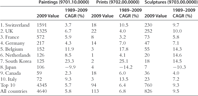
Shown are nominal US exports and annual growth rates by country and HS10 category. CAGR, compound annual growth rate.
Source: USITC and author calculations.
Table 10.3 documents the same statistics for US imports of paintings, prints, and sculptures. Again, we see a high degree of concentration in the top 10 countries and, within those, the top four. In contrast to exports, however, we do not observe a strong link between the export growth rates of foreign economies and their rates of overall output growth. For instance, top exporters such as Italy and Spain did not register particularly high GDP growth over this period, while the growth rate of Japanese sculpture exports was actually above average. We also do not observe as strong a correlation in growth rates across products for a given country. Taken together, US export and import statistics suggest that importer GDP plays a more determinate role in art trade flows than exporter GDP.
Table 10.3
US imports of visual arts, 1989–2009 (nominal, $ millions).
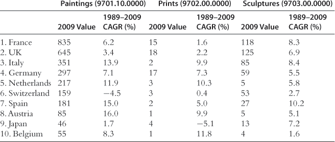
Shown are nominal US imports and annual growth rates by country and HS10 category. CAGR, compound annual growth rate.
Source: USITC and author calculations.
Since the art trade values are measured in nominal terms, the statistics computed in Tables 10.2 and 10.3 conflate growth in both quantities and prices. To properly measure the real services embodied in paintings, prints, and sculptures, an appropriate deflator should be applied. Information on art prices can be gleaned from a variety of sources in the empirical art literature and we will additionally suggest a new source of art prices from the international trade data. Figure 10.1 shows the evolution of two hedonic indexes for paintings estimated by Renneboog and Spaenjers (2013). Much popular interest in art as an investment has stemmed from the observation that painting prices, driven largely by prices for oil paintings, have climbed considerably since 2001, re-attaining levels last seen in the late 1980s. While Renneboog and Spaenjers use a large amount of auction data and a hedonic methodology to come up with their index, we can garner additional information on art prices from sources that are perhaps less careful about art quality and vintage though even more broad in their coverage of collectible items. Those sources include government statistical agencies that collect price data on international transactions. For example, the US Bureau of Labor Statistics (BLS) International Price Program (IPP) surveys a sample of US importing and exporting firms to construct indexes of prices for traded goods. Given the international nature of art markets as well as the geographic concentration of sellers, we might expect that goods crossing a popular border like that of the United States would provide a more-or-less representative sample of current transactions. Indeed when we look at US import prices from the IPP for the product category Coins, Gems, Jewelry, and Collectibles (three-digit End Use product code 413), we see that much of the recent dynamic in markets for paintings is captured by the broader index of collectibles.8 It is rather remarkable that painting prices are so similar to those of collectible goods, many of which we would not consider to be a class of investment. In the following analyses, the art trade volume data will be deflated by these indexes to obtain a measure of real art exports.

Figure 10.1 Painting and collectible prices. Source: US BLS and Renneboog and Spaenjers (2013).
10.4 The Correlation Between Exports of Artworks, Consumer Goods, and Capital Goods
Do fine art exports look more like consumption or investment goods? A sensible empirical starting point is to take the US Bureau of Economic Analysis (BEA)’s definitions of broad sector categories and to examine the extent to which art trade coincides with contemporaneous bilateral exports in those sectors. Of particular relevance will be the correlation of art exports with exports of consumer goods and capital goods, where the former is a proxy for consumption demand and the latter is more closely related to investment demand.9 The consumer goods category does indeed contain many subcategories that can be regarded as final goods intended for consumption such as household goods, recreational equipment, home entertainment, coins, gems, and jewelry.10 The capital goods category contains goods more typically associated with business investment such as electricity generation equipment, industrial and agricultural machinery, computers, business machines, aircraft, and other vessels.
Figure 10.2 shows an index of real US exports of paintings compared to those of four large sectors. The paintings index is deflated using the RS Oil price series from Fig. 10.1, extended through 2010q1 using the growth rates of the BLS collectibles index. Each of the major goods categories is deflated by its own corresponding export price index as constructed by the BLS. With the exception of a surge and decline in real painting exports in the late 1980s, all series are characterized by relatively steady growth through the 1990s. The series then diverge rather dramatically during the 2000s, with foods, feeds, and beverages, and industrial supplies growing modestly, well below accelerating exports of automotive and capital goods. Paintings experienced another surge and contraction in exports in the early 2000s and then followed consumer goods’ brisk upward trajectory thereafter. Exports of all goods plunged in the wake of the financial crisis in late 2008, though signs of recovery were evident in all sectors except paintings by early 2010. Interestingly, in addition to being closely linked to the growth of the real exports of consumer goods, the real painting export series is highly countercyclical, surging during periods of US recession.

Figure 10.2 Real US painting exports relative to other sectors. Source: US export volume data are published by US BEA and US ITC. Price series used as deflators are from the US BLS.
We proceed to quantify these correlations conditioning further on destination country, global shocks and seasonal patterns in the following reduced-form least-squares regression:
![]() (10.2)
(10.2)
where Mjkt is the nominal flow of US exports of art HS10 product j, to country k in year t. Depending on the specification, the vector of zs contains either dummy variables for the time period or for the destination country, controlling for the global levels and destination-specific features of US exports respectively. To avoid issues of seasonality, we implement the regression on annual data ranging from 2002 to 2009.11 Table 10.4 shows the resulting estimates for αs across an array of specifications for each of painting, print, and sculpture exports. The first two columns in each product category show the results using year- and destination-fixed effects, respectively. Additionally, to allay concerns that the series are not stationary and hence give rise to spurious positive correlations, we rerun the estimation in first differences under the alternative hypothesis that the series are difference stationary. The results of these regressions in first differences are shown in the third column for each product.
Table 10.4
The correlation of US art exports with aggregate sector exports (nominal).

Each column shows the log of annual bilateral US art exports regressed on the log of aggregate US exports by broad sector for the years 2002–2009. Consumer goods exports are net of painting, print, and sculpture sales. Standard errors are shown in parentheses. Significant at the *10%, **5%, and ***1% level.
Table 10.4 indicates that the flows of artworks do not tend to be systematically correlated with any category except consumer goods. In particular, art exports are positively and significantly correlated with consumer goods exports in most products and specifications, with elasticities ranging from about 0.5 to 2. These estimates imply that when consumer goods exports increase by 10% to a given destination, art exports increase by 5–20%. Capital goods, on the other hand, have only one estimate that is statistically different from zero (the correlation with sculpture exports) and it is negative. Industrial supplies, foods, feeds, and beverages, and automotive products have a few sporadic estimates that are statistically significant, though those are split between positive and negative correlations.
The international trade data in Table 10.4 are nominal flows, and hence conflate price and quantity changes; correlated inflation rates for art and consumption goods could be contributing to the results. In Table 10.5, as well as the empirical applications below, the art trade data are deflated by various price series to generate measures of real flows. These are the appropriate units with which to measure consumption versus investment demand. Given the information at hand on art prices, we deflate each series by its corresponding index and evaluate the correlation between real art exports and the real exports of the major sectors. Ideally one would like to deflate each destination-specific trade flow; however, price indexes at that level of detail are not available. Nonetheless, deflating by the sector-specific deflator removes the influence of the average price level across destinations. Table 10.5 shows an analogous set of estimates to Table 10.4, though in real terms. Again, art exports are highly correlated with consumer goods exports and not systematically related to the exports of other sectors.
Table 10.5
The correlation of US art exports with aggregate sector exports (real).
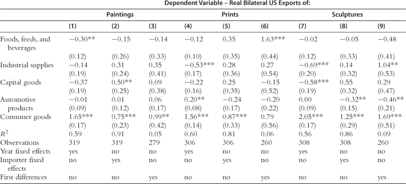
Each column shows the log of annual bilateral US art exports regressed on the log of aggregate US exports by broad sector for the years 2002–2009. Consumer goods exports are net of painting, print, and sculpture sales. Standard errors are shown in parentheses. Significant at the *10%, **5%, and ***1% level.
Although these results suggest that arts are demanded more for consumption services than investment services, certain caveats are in order. Importantly, using capital goods as a measure of investment demand may not be completely appropriate since it proxies for real investment demand, not financial investment demand. Moreover, the demand for capital goods by firms is presumably driven by many other factors besides the consumption smoothing behavior of the firm’s owners; it will depend on the firm’s technology, the quantities of other inputs in production, and also the idiosyncrasies of capital markets. Ideally, what one would like to identify in the data is a pure measure of savings demand. The following sections use the logic of the PIH to that end.
10.5 Art Trade and Permanent Income
In this section, we continue to explore the fundamental question of whether art is demanded for its consumption or investment services, developing an empirical test based on Milton Friedman (1957) PIH. The PIH offers a stylized behavioral prediction based on whether shocks to wealth are permanent or transient; agents in an economy will consume all of a permanent shock and save most of a transient one. Through this lens, the correlation of real US art exports with permanent and transient income changes abroad is informative about the underlying motives of foreign art buyers. The following subsections suggest two different decompositions of foreign GDP changes into permanent and temporary components, and we shall see the extent to which each of these components varies with international art purchases.
10.5.1 PIH Predictions in a State-Space Model
First of all, our test of the PIH predictions also requires data measures of temporary and permanent income innovations. Our empirical decomposition of real GDP into these two components follows Clark (1987) and applies the unobserved-components econometric model. The idea in this class of models is to specify a measurement equation describing the relationship between observed data and unobserved state variables, and a transition equation describing the dynamics of the state variable. The analysis then uses the Kalman filter to estimate the unobserved component of the state variable using information available at any given time t. A common application of this estimation technique is to decompose the log of GDP into a stochastic trend component and a cyclical component. Following the exposition of Clark (1987) in Kim and Nelson (1999), we specify the following unobserved components model:
 (10.3)
where y is the log of real GDP for a given country, x is a stationary cyclical component, and n is the stochastic trend (i.e. permanent) component (IID = independent and identically distributed). There is a drift term, g, which is modeled as a random walk. This system of equations and its state-space representation are estimated for each country to recover the cyclical dynamics (θ) as well as the variance of each innovation (σ). With these estimates we can construct series for x and n for each country. As an illustration, Fig. 10.3 shows the resulting decomposition for the United Kingdom. We see that the permanent component has risen steadily since 1993, with more rapid growth in the 1990s than the 2000s. The cyclical component is, by construction, stationary about zero; that series has four peaks with the most recent one preceding the financial crisis of 2008/09.

To implement the PIH test, the correlations between changes in bilateral real art flows and changes in the components of real GDP are estimated. We implement these predictions by running the following least-squares regression:12
![]() (10.4)
(10.4)
where M is the flow of nominal US exports of product j (paintings, prints, or sculptures) to country k at time t deflated by an index of art prices (Pt).13 The changes in the real GDP of importing nations are of three types: overall, temporary, and permanent.
As above, real art imports are measured at the quarterly frequency for each of the three HS 10-digit products: paintings, prints, and sculptures. Nominal imports are deflated by the import price index computed by the BLS for the three-digit End Use product 413: Coins, gems, jewelry, and collectibles, from Fig. 10.1.14 On the right-hand side, seasonally adjusted real GDP for 32 countries is obtained at the quarterly frequency from Haver (www.haver.com), and decomposed into temporary and permanent components as described above. In one of the specifications below, we will use an alternative measure of international investment demand from the US Treasury International Capital (TIC) system. TIC data document monthly US transactions in long-term securities and we will use ‘Gross Sales by US Residents to Foreigners’ of US stocks and treasury bonds, aggregated to the quarterly frequency, as a measure of foreign investment demand.
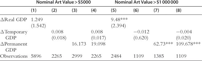
Table 10.6 shows the baseline estimates of α1. The left panel (columns (1)–(4)) includes all bilateral quarterly flows greater than $5000, a total of just over 6000 observations. In column (1), a 1% increase in national real GDP translates into a 3.4% increase in contemporaneous art imports, significant at the 5% level. An elasticity of above 1 implies that the share of art in income is increasing over time, which suggests that art is either a superior consumption good or becoming an increasingly attractive investment. Decomposing this coefficient into permanent and temporary components in columns (2)–(4), we see that there is little discernible correlation between the temporary component of income changes and art imports, while the permanent component is very strongly correlated with art purchases – a 1% increase in the permanent component of income increases art purchases by 24%. That permanent innovations in income stimulate art purchases while temporary innovations do not is consistent with the PIH prediction that art is a consumption good and not an investment.
Table 10.6
The elasticity of real artwork exports to temporary and permanent innovations in foreign GDP.
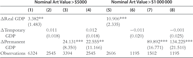
The dependent variable is the real bilateral US export value of paintings, prints, and sculptures. Standard errors are shown in parentheses. Significant at the 5% (**) and 1% (***) level.
In the right panel, the regressions are rerun only for countries whose art imports for a product within a given quarter exceeded $1 million. It is immediately apparent that all of the estimated coefficients are magnified. The overall responsiveness of art imports to GDP for this subset is 11%. While the response of art purchases to temporary income innovations is still zero, the elasticity of purchases with respect to permanent innovations increases to a staggering 89%. Therefore, it is not just that art behaves like a consumption good, it is also that the correlation of income and art demand is concentrated in countries with relatively high levels of quarterly purchases. This observation could be driven by a number of factors. Countries with higher levels are likely wealthier, have a larger proportion of art consumers and have ‘deeper ties’ to art markets; all of these factors might contribute to import flows being more sensitive to income.
Tables 10.7 and 10.8 explore the hypothesis that art demand changes with income relative to other consumption and investment goods. Recall that these correlations are informative about the type of a given consumption good or investment vehicle. In Table 10.7, the dependent variable is the quarterly change in real art exports from the United States, again at the HS10 level, normalized by the total amount of US exports to each country in a given period. For example, in the first quarter of 2009 Germany imported $530 million worth of paintings from the United States, a 39% decline relative to the previous year; over the same period real GDP in Germany was down about 6%. However, the decline in art purchases is less pronounced relative to total German imports from the United States, which dropped by 17%, than it is to total GDP. In other words, it is important to additionally control for factors that affect overall trade flows. In this example, we find that art demand is sensitive to income at a rate of greater than one-for-one, even after controlling for total imports as a gauge of other consumption goods. As such, art consumption is not only increasing relative to income but increasing as a share of all goods. This pattern is supported by the data, albeit with low statistical significance. In the left panel of Table 10.7 we find that art imports behave much like superior consumption goods – the relative consumption of artworks increases with income, specifically with permanent increases in income. The right panel, looking at the large importer set, is more precisely estimated with an elasticity of art imports to permanent GDP of 63. This suggests that much of the increase in the consumption of art in the wake of an innovation to income is a relative increase.
Table 10.7
The elasticity of real artwork export share to temporary and permanent innovations in foreign GDP.
The dependent variable is the real bilateral US export value of paintings, prints, and sculptures as a share of total bilateral exports. Standard errors are shown in parentheses. Significant at the 5% (**) and 1% (***) level.
Table 10.8
The elasticity of real artwork exports to temporary and permanent innovations in foreign GDP, controlling additionally for foreign asset purchases.

Notes: The dependent variable is the real bilateral U.S. export value of paintings, prints and sculptures. Standard errors shown in parentheses. Significant at the 5% (**) and 1% (***) level.
Table 10.8 shows the analogous results for investment flows using TIC data for US stocks and treasury bonds. The dependent variable is the quarterly change in real product-level art exports (similar to Table 10.6), but we now include an additional control for the quarterly change in bilateral foreign purchases of US securities on the right-hand side. The coefficients on the TIC variables tell us whether art flows are correlated with investment flows, for example whether German purchases of US stocks rise and decline in tandem with art purchases. We find only weak evidence that art flows are related to the nominal flows of these investment goods. For a 1% increase in foreign purchases of US treasury bonds, art imports rise by a modest 0.14%, significant at the 5% level, while art flows are uncorrelated with foreign purchases of US equities.
Finally, we use the data on aggregate bilateral international investment to check that the PIH predictions hold for purchases of products that we know to be either investments or consumption goods. Table 10.9 shows the results of regressions of the form:
![]() (10.5)
(10.5)
where Z is the nominal flow of a given investment (i.e. stocks and T-bills) or consumption product (i.e. aggregate trade flows). In columns (1)–(3), the dependent variable is the bilateral foreign purchase of US stocks. If stocks are pure investments, then the PIH would predict that their purchase is correlated with temporary innovations to GDP, though less so for permanent ones. We find that foreign purchases of US equities are indeed correlated with temporary and permanent changes to real GDP. T-bills in columns (4)–(6) behave much like the canonical PIH investment vehicle – they are strongly correlated with temporary innovations to GDP, but with a coefficient indistinguishable from zero on the permanent innovations. In columns (7)–(9), aggregate trade flows (e.g. all of the US exports to Germany) are positively correlated with both the temporary and permanent components of GDP, with a much stronger correlation with the permanent component. This observation conforms to one’s prior notions about the composition of trade: most of it is likely for consumption, but with some of it being accounted for by investment.
Table 10.9
The elasticity of nominal asset and aggregate trade flows to temporary and permanent innovations in foreign GDP.

The dependent variable is the real bilateral US export value of paintings, prints, and sculptures as a share of total bilateral exports. Standard errors are shown in parentheses. Significant at the 5% (**) and 1% (***) level.
As an additional robustness check, we can investigate the possibility that income may operate with a lag on art purchases. In Table 10.10 the baseline results are reproduced with four-quarter lags of the independent variables, yielding results that are quite similar.
Table 10.10
The elasticity of real artwork exports to temporary and permanent innovations in foreign GDP (lagged independent variables).

The dependent variable is the real bilateral US export value of paintings, prints, and sculptures. Standard errors are shown in parentheses. Significant at the 5% (**) and 1% (***) level.
10.5.2 PIH Predictions in a Structural VAR Model
A different method for identifying permanent income innovations is developed in the literature on RBCs. The dynamics in the canonical RBC model are driven by shocks to the technology parameter in production, which in turn have first-order effects on the level of national output and income. Gali (1999) evaluates the conditional correlations of the model in national data using an identification strategy that distinguishes technology from non-technology drivers of productivity and employment. The intuition of that strategy is that only permanent changes in the stochastic technology parameter can be the source of a unit root in productivity. In other words, the high degree of persistence of labor productivity is driven by the high degree of persistence in the underlying technology process, and not by other factors which can have only a transient impact. For our purposes, a permanent technology shock is tantamount to a permanent innovation in income. Thus, we can mimic Gali’s strategy and measure the conditional correlation of art demand with permanent income as measured by a technology shock. Again, the PIH will associate a positive conditional correlation with the consumption for art purchases.15
Following Gali, we specify the following bivariate system for national labor productivity (Xkt) and US real bilateral art exports:
 (10.6)
where the left-hand side vector is assumed to be I(1) with a stationary VAR representation in first differences. The right-hand side is a distributed lag of disturbances of technology (![]() ) and non-technology (
) and non-technology (![]() ) components, which are allowed to vary by country. Gali’s identifying assumption above is implemented as
) components, which are allowed to vary by country. Gali’s identifying assumption above is implemented as ![]() (i.e. the only source of permanent fluctuations in labor productivity is
(i.e. the only source of permanent fluctuations in labor productivity is ![]() ). Under the assumptions that the technology and non-technology disturbances are orthogonal to one another, and that the reduced form VAR innovations are a linear combination of those disturbances, we can consistently estimate
). Under the assumptions that the technology and non-technology disturbances are orthogonal to one another, and that the reduced form VAR innovations are a linear combination of those disturbances, we can consistently estimate ![]() and the corresponding impulse response functions for technology and non-technology shocks. A positive increase in real art exports following a foreign technology shock is indicative that art is a consumption good.
and the corresponding impulse response functions for technology and non-technology shocks. A positive increase in real art exports following a foreign technology shock is indicative that art is a consumption good.
Data for national labor productivity are the log differences of quarterly, seasonally adjusted output per worker-hour for each of the top four destination markets of US art exports: Switzerland, the United Kingdom, France and Germany.16 Again, the real art export flows are the nominal US export volumes to each country deflated by the BLS price index for collectibles. The impulse responses of painting, print, and sculpture purchases to technology shocks (i.e. permanent income shocks) are shown for these importers in Figs. 10.A1–10.A3 in the Appendix. Also shown are bootstrapped 90% confidence bands for the impulse responses. The estimates tend to reinforce the fact that art responds to permanent income. For paintings, the estimates of export response to the United Kingdom, Germany, and France are positive upon impact of the permanent income shock. For the United Kingdom and France, in particular, permanent income innovations lead to increases in art purchases of around $7 million and $4 million per quarter, respectively, for each percentage point increase in productivity. For prints, the results are decidedly weaker with none of the shocks registering significant changes on impact and with several of the estimates below zero. For sculptures, there are several positive estimates on impact, with the increase significantly different from zero for France. Overall, the balance of correlation estimates between permanent income and art purchases is positive for the larger painting and sculpture categories. However, this result is qualified by the lack of response in prints and, in some instances, our inability to reject the null hypothesis of no effect.


10.6 Concluding Remarks
This chapter presents an exploration of the flows and dynamics of the international markets for paintings, prints, and sculptures. In contrast to the bulk of previous studies, our focus has been on the real flows of art purchases, which, as opposed to prices alone, provide a more complete measure of the flow of real services from visual arts. Using a battery of novel measures, we have seen that these services most closely resemble consumption services. International art trade varies closely with trade in consumer goods, with the income of destination countries, and specifically with the permanent component of income innovations. In contrast, there is little indication that art demand responds to temporary income shocks or that it even moves in tandem with other investment vehicle flows, suggesting that the investment motive for purchasing art is relatively weak. The interpretation of the results is also robust to variations in country characteristics. For instance, countries with larger, more stable art flows exhibit stronger correlations with permanent income – a result consistent with the notion that information flows and networks play key roles in the export success of these highly distinctive goods. Moreover, the high concentration of art importers and the persistence of this concentration over time suggest that it is indeed the incumbent market participants driving the results rather than the entry and exit of new art-importing countries.
Certain qualifications are in order for the pre-eminence of consumption versus investment motives in buying art. (i) The effects identified here are average effects within and across countries. Using country data, it is difficult to reject the hypothesis that a portion of the art-buying population is composed of ‘pure’ investors. The distributional characteristics of art buyers and returns are investigated more thoroughly in Goetzmann et al. (2012) and Scorcu and Zanola (2010). Further, looking at country averages likely smoothes over differences in the balance of consumers and investors. The trade data suggest, however, that the average art buyer is a consumer. (ii) The focus on international data ignores a possible selection bias of traded visual arts versus art consumed domestically. While the characteristics of cross-border art purchases relative to domestic ones is beyond the scope of this study, one might conjecture that in order to bear the higher costs of international transactions such as taxes, shipping, or marketing, international sales are predominantly up-market sales. If true, the selection induced by only considering international trade would be consistent with previous studies that have found masterpieces to be poor investments. (iii) It is important to acknowledge that fine art is quite distinct from other traded goods because of the manner in which art is sold, primarily through auctions. Here, we have abstracted from the idiosyncrasies and vagaries of auctions, such as those identified in Ashenfelter and Graddy (2006), but are cognizant of the possibility that the process of selling visual art may itself be a function of the state of the economy and hence a factor in determining trade flows.
Acknowledgments
The author thanks Seth Pruitt for providing the MATLAB code of the unobserved components model, as well as Joseph Gruber, David Throsby, Robert Vigfusson, and participants in sessions at the Association for Cultural Economics International 2010 and Southern Economic Association 2011 conferences for helpful comments. Nathaniel Dau-Schmidt and Mallory Nobles provided excellent research assistance. The views in this chapter are solely the responsibility of the author and should not be interpreted as reflecting the views of the Federal Reserve Bank of New York or the Federal Reserve System.
Appendix
Table 10.A1 shows US trade data categories for visual art HS codes. Table 10.A2 lists categories that are not included in the definition of visual art.
Table 10.A1
US trade data categories for visual art: visual art is classified as the following US HS products.
| HS Code | Description | |
| Paintings | 9701.10.0000 | Paintings, drawings and pastels other than of heading 4906 |
| Prints | 9702.00.0000 | Original engravings, prints and lithographs, framed or not framed |
| Sculptures | 9703.00.0000 | Original sculptures and statuary, in any material |
Table 10.A2
Categories not included in the definition of visual art.
| Paintings | |
| 4906 | Plans and drawings for architectural, engineering, industrial, commercial, topographical or similar purposes, originals, and specific reproductions |
| 5805.00 | Hand-woven tapestries of the type Gobelins, Flanders, Aubusson, Beauvais, and the like, and needle-worked tapestries (e.g. petit point, cross stitch), whether or not made up |
| 5907.00 | Textile fabrics otherwise impregnated, coated, or covered; painted canvas being theatrical scenery, studio back-cloths, or the like: other made up textile articles; sets; worn clothing and worn textile articles; rags |
| 6304.99.1000 | Certified hand-loomed and folklore products |
| 6304.99.2500 | Wall hangings of jute |
| 9701.90.0000 | Painting, drawing and pastels, NESOI |
| 9810.00.1000 | Painted, colored, or stained glass windows and parts thereof, all the foregoing valued over $161 per square meter and designed by, and produced by or under the direction of, a professional artist |
| Prints | |
| 4911.91 | Pictures, designs, and photographs |
| 4911.91.20 | Lithographs on paper or paperboard not over 0.51 mm in thickness |
| 4911.91.2020 | Posters |
| Sculptures | |
| 4420.10.0000 | Statuettes and other ornaments, of wood |
| 6913.10 | Statuettes and other ornamental ceramic articles, of porcelain or china |
| 6913.10.1000 | Statues, statuettes, and handmade flowers, valued over $2.50 each and produced by professional sculptors or directly from molds made from original models produced by professional sculptors |
| 8306.10.0000 | Bells, gongs, and the like, and parts thereof; statuettes and other ornaments, and parts thereof |
| 9601 | Worked ivory, bone, tortoise-shell, horn, antlers, coral, mother-of-pearl, and other animal carving material, and articles of these materials (including articles obtained by molding) |
Figures 10.A1–10.A3 show estimated impulse responses of real US painting, print, and sculpture exports to a permanent income shock.
References
1. Ashenfelter O, Graddy K. Auctions and the price of art. Journal of Economic Literature. 2003;41:763–787.
2. Ashenfelter O, Graddy K. Art auctions. In: Amsterdam: North-Holland; 2006;909–946. Ginsburgh VA, Throsby D, eds. Handbook of the Economics of Art and Culture. vol. 1.
3. Baumol WJ. Unnatural value: or art investment as floating crap game. American Economic Review. 1986;76:10–14.
4. Baumol WJ, Throsby D. Psychic payoffs, overpriced assets, and underpaid superstars. Kyklos. 2012;65:313–326.
5. Clark PK. The cyclical component of US economic activity. Quarterly Journal of Economics. 1987;102:797–814.
6. Dimson E, Spaenjers C. Ex post: the investment performance of collectible stamps. Journal of Financial Economics. 2011;100:443–458.
7. Friedman M. A Theory of the Consumption Function. Princeton, NJ: Princeton University Press; 1957.
8. Gali J. Technology, employment, and the business cycle: do technology shocks explain aggregate fluctuations? American Economic Review. 1999;89:249–271.
9. Ginsburgh V, Mei J, Moses M. The computation of prices indices. In: Amsterdam: North-Holland; 2006;947–979. Ginsburgh VA, Throsby D, eds. Handbook of the Economics of Art and Culture. vol. 1.
10. Goetzmann WN, Renneboog L, Spaenjers C. ‘Art and money’. American Economic Review Papers and Proceedings. 2012;101:222–226.
11. Graddy K, Margolis P. Fiddling with value: violins as an investment? CEPR Discussion Paper 6583. London: Centre for Economic Policy Research; 2007.
12. Kim C-J, Nelson CR. State-Space Models with Regime Switching: Classical and Gibbs-Sampling Approaches with Applications. Cambridge, MA: MIT Press; 1999.
13. Locatelli-Biey M, Zanola R. The sculpture market: an adjacent year regression index. Journal of Cultural Economics. 2002;26:65–78.
14. Mandel BR. Art as an investment and conspicuous consumption good. American Economic Review. 2009;99:1653–1663.
15. Pesando JE. Art as an investment: the market for modern prints. American Economic Review. 1993;83:1075–1089.
16. Pesando JE, Shum PM. The returns to Picasso’s prints and to traditional financial assets, 1977 to 1996. Journal of Cultural Economics. 1999;23:181–190.
17. Pesando JE, Shum PM. The auction market for modern prints: confirmations, contradictions, and new puzzles. Economic Inquiry. 2008;46:149–159.
18. Pownall, R.A.J. (2007). ‘Art as a financial investment’. Working Paper. Tilburg University, Tilburg. Available form SSRN: <http://ssrn.com/abstract=978467>.
19. Renneboog L, Spaenjers C. Buying beauty: on prices and returns in the art market. Management Science. 2013;59:36–53.
20. Sagot-Duvauroux D. Art prices. In: Towse R, ed. A Handbook of Cultural Economics. Cheltenham: Edward Elgar; 2011;43–48.
21. Scorcu, A.E., Zanola, R (2010). ‘The ‘right’ price for art collectibles. A quantile hedonic regression investigation of Picasso paintings’. Working Paper Series 01_10. Rimini Centre for Economic Analysis, Rimini.
22. Throsby D. The production and consumption of the arts: a view of cultural economics. Journal of Economic Literature. 1994;32:1–29.
23. Velthuis O. Talking Prices: Symbolic Meanings of Prices on the Market for Contemporary Art. Princeton NJ: Princeton University Press; 2005.
1This argument assumes that all traded goods are a form of consumption good. If some imports (such as capital goods) are in fact investments, then the sensitivity of the art share to a permanent income innovation would be lower.
2For more information on the collection and compilation of US trade data, as well as for statistics updated monthly, see: www.census.gov/foreign-trade/index.html.
3Generally, information is also available on physical quantities of items imported and exported. However, unfortunately, for the fine art categories those data are not made available.
4HS codes are comparable across countries at the six-digit level. The extra four digits are particular to the description of US traded goods. The 10-digit codes are also referred to collectively as the Harmonized Tariff Schedule.
5For a detailed list of HS10 product categories that are not included in the definition of fine art, see Table 10.A2 in the Appendix.
6The US Census Bureau is careful to count only sales in its export data. If there is a reasonable expectation that a good is not being sold, it is excluded from the trade records. Such a situation might arise, for example, if galleries or museums are transferring artworks on loan, if auction houses are sending an unsold work to a foreign affiliate, or if private individuals are moving their collection without a change in ownership.
7The compound annual growth rates are a few percentage points higher if we instead compute them over the period ending in 2008. However, the other patterns are qualitatively similar.
8The poor performance of the BLS index in capturing the large decline in art prices at the beginning of the sample period may reflect changes in the IPP sampling and index construction protocol, which evolved considerably during the 1990s. For further information on how IPP constructs its price indexes, see the BLS Handbook of Methods, published online at: http://www.bls.gov/opub/hom/.
9The BEA categorizes goods trade according to the End Use classification scheme at the one-digit sector level.
10Artworks are classified as consumer goods by the BEA and thus what we refer to as consumer goods hereafter is the BEA measure, net of a smoothed series for paintings, prints, sculptures, stamps, and antiques.
11Sectoral US export data by country were downloaded from the BEA.
12Since the permanent component of GDP is typically non-stationary, the dataset is first converted to first differences.
13Due to data limitations on prices, it is assumed that the deflator is common among products and destination countries.
14No US export price index is available for this product category. However, as shown above, the price deflator does a good job of tracking price movements in an international auction-based painting index. For this exercise, the trade price index is slightly favored since it encompasses more products and is particular to the selection of artworks traded internationally. The results are not qualitatively different if instead we use the painting index as the deflator.
15A zero or negative correlation is not necessarily due to the investment motive for purchasing art, since we have not identified a temporary innovation in technology. Temporary changes to the technological process will affect labor productivity along with many other factors and, hence, they are more difficult to isolate.
16Productivity data by country was downloaded from Haver (www.haver.com).