
1
An overview of data mining: The applications, the methodology, the algorithms, and the data
1.1 The applications
Customers are the most important asset of an organization. That’s why an organization should plan and employ a clear strategy for customer handling. Customer relationship management (CRM) is the strategy for building, managing, and strengthening loyal and long-lasting customer relationships. CRM should be a customer-centric approach based on customer insight. Its scope should be the “personalized” handling of the customers as distinct entities through the identification and understanding of their differentiated needs, preferences, and behaviors.
CRM aims at two main objectives:
- Customer retention through customer satisfaction
- Customer development
Data mining can provide customer insight which is vital for these objectives and for establishing an effective CRM strategy. It can lead to personalized interactions with customers and hence increased satisfaction and profitable customer relationships through data analysis. It can offer individualized and optimized customer management throughout all the phases of the customer life cycle, from acquisition and establishment of a strong relationship to attrition prevention and win-back of lost customers. Marketers strive to get a greater market share and a greater share of their customers. In plain words, they are responsible for getting, developing, and keeping the customers. Data mining can help them in all these tasks, as shown in Figure 1.1.
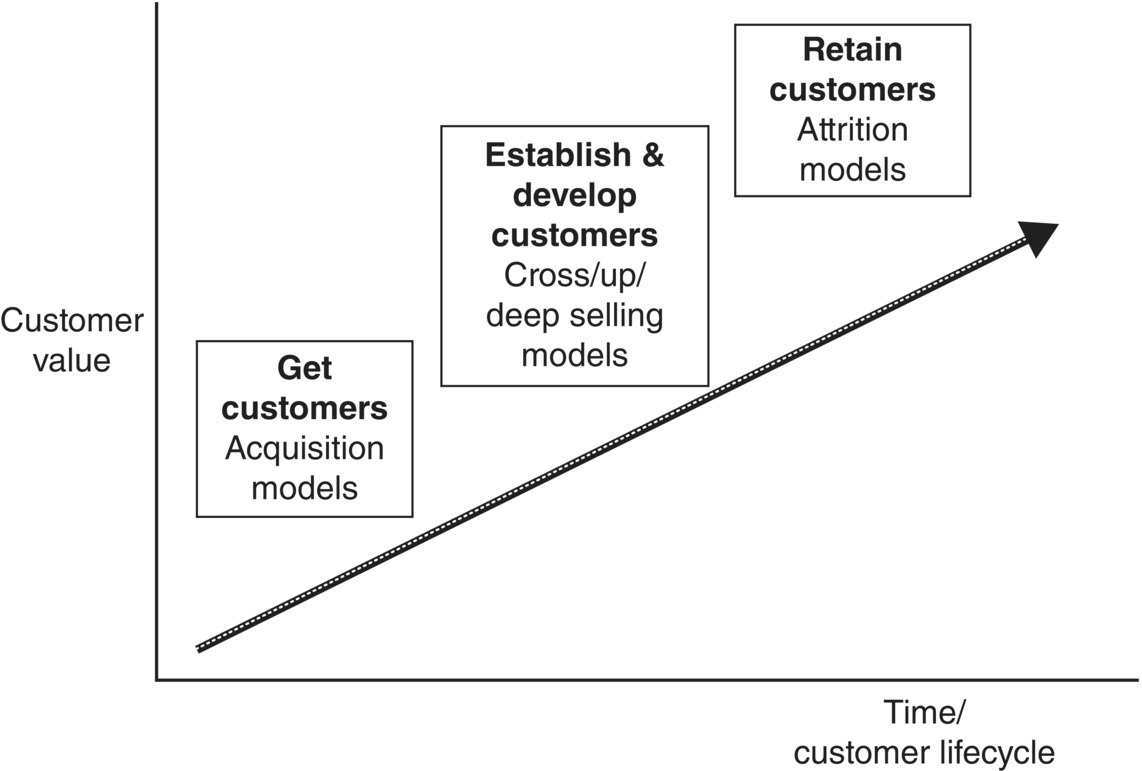
Figure 1.1 Data mining and customer life cycle management.
Source: Tsiptsis and Chorianopoulos (2009). Reproduced with permission from Wiley
More specifically, the marketing activities that can be supported with the use of data mining include:
Customer segmentation
Segmentation is the process of dividing the customer base in distinct and homogeneous groups in order to develop differentiated marketing strategies according to their characteristics. There are many different segmentation types according to the specific criteria/attributes used for segmentation. In behavioral segmentation, customers are grouped based on behavioral and usage characteristics. Although behavioral segments can be created using business rules, this approach has inherent disadvantages. It can handle only a few segmentation fields, and its objectivity is questionable as it is based on the personal perceptions of a business expert. Data mining on the other hand can create data-driven behavioral segments. Clustering algorithms can analyze behavioral data, identify the natural groupings of customers, and suggest a grouping founded on observed data patterns. Provided it is properly built, it can uncover groups with distinct profiles and characteristics and lead to rich, actionable segmentation schemes with business meaning and value.
Data mining can also be used for the development of segmentation schemes based on the current or expected/estimated value of the customers. These segments are necessary in order to prioritize the customer handling and the marketing interventions according to the importance of each customer.
Direct marketing campaigns
Marketers carry out direct marketing campaigns to communicate a message to their customers through mail, Internet, e-mail, telemarketing (phone), and other direct channels in order to prevent churn (attrition) and drive customer acquisition and purchase of add-on products. More specifically, acquisition campaigns aim at drawing new and potentially valuable customers from the competition. Cross/deep/up-selling campaigns are rolled out to sell additional products, more of the same product, or alternative but more profitable products to the existing customers. Finally, retention campaigns aim at preventing valuable customers from terminating their relationship with the organization.
These campaigns, although potentially effective, when not refined can also lead to a huge waste of resources and to the annoyance of customers with unsolicited communication. Data mining and classification (propensity) models in particular can support the development of targeted marketing campaigns. They analyze the customer characteristics and recognize the profile of the target customers. New cases with similar profiles are then identified, assigned a high propensity score, and included in the target lists. Table 1.1 summarizes the use of data mining models in direct marketing campaigns.
Table 1.1 Data mining models and direct marketing campaigns
Source: Tsiptsis and Chorianopoulos (2009).
| Business objective | Marketing campaign | Data mining models |
| Getting customers |
|
|
| Developing customers |
|
|
| Retaining customers |
|
|
When properly built, propensity models can identify the right customers to contact and lead to campaign lists with increased concentrations of target customers. They outperform random selections as well as predictions based on business rules and personal intuitions.
Market basket and sequence analysis
Data mining and association models in particular can be used to identify related products, typically purchased together. These models can be used for market basket analysis and for the revealing of bundles of products/services that can be sold together. Sequence models take into account the order of actions/purchases and can identify sequences of events.
1.2 The methodology
The modeling phase is just one phase in the implementation process of a data mining project. Steps of critical importance precede and follow the model building and have a significant effect in the success of the project. An outline of the basic phases in the development of a data mining project, according to the Cross Industry Standard Process for Data Mining (CRISP-DM) process model, is presented in Table 1.2.
Table 1.2 The CRISP-DM phases
Source: Tsiptsis and Chorianopoulos (2009). Reproduced with permission from Wiley.
| 1. Business understanding | 2. Data understanding | 3. Data preparation |
|
|
|
| 4. Modeling | 5. Model evaluation | 6. Deployment |
|
|
|
Data mining projects are not simple. They may end in business failure if the engaged team is not guided by a clear methodological framework. The CRISP-DM process model charts the steps that should be followed for successful data mining implementations. These steps are:
- Business understanding. The data mining project should start with the understanding of the business objective and the assessment of the current situation. The project’s parameters should be considered, including resources and limitations. The business objective should be translated to a data mining goal. Success criteria should be defined and a project plan should be developed.
- Data understanding. This phase involves considering the data requirements for properly addressing the defined goal and an investigation on the availability of the required data. This phase also includes an initial data collection and exploration with summary statistics and visualization tools to understand the data and identify potential problems of availability and quality.
- Data preparation. The data to be used should be identified, selected, and prepared for inclusion in the data mining model. This phase involves the data acquisition, integration, and formatting according to the needs of the project. The consolidated data should then be cleaned and properly transformed according to the requirements of the algorithm to be applied. New fields such as sums, averages, ratios, flags, etc. should be derived from the original fields to enrich the customer information, better summarize the customer characteristics, and therefore enhance the performance of the models.
- Modeling. The processed data are then used for model training. Analysts should select the appropriate modeling technique for the particular business objective. Before the training of the models and especially in the case of predictive modeling, the modeling dataset should be partitioned so that the model’s performance is evaluated on a separate validation dataset. This phase involves the examination of alternative modeling algorithms and parameter settings and a comparison of their performance in order to find the one that yields the best results. Based on an initial evaluation of the model results, the model settings can be revised and fine-tuned.
- Evaluation. The generated models are then formally evaluated not only in terms of technical measures but, more importantly, in the context of the business success criteria set in the business understanding phase. The project team should decide whether the results of a given model properly address the initial business objectives. If so, this model is approved and prepared for deployment.
- Deployment. The project’s findings and conclusions are summarized in a report, but this is hardly the end of the project. Even the best model will turn out to be a business failure if its results are not deployed and integrated in the organization’s everyday marketing operations. A procedure should be designed and developed that will enable the scoring of customers and the update of the results. The deployment procedure should also enable the distribution of the model results throughout the enterprise and their incorporation in the organization’s data warehouse and operational CRM system. Finally, a maintenance plan should be designed and the whole process should be reviewed. Lessons learned should be taken into account and next steps should be planned.
The aforementioned phases present strong dependencies, and the outcomes of a phase may lead to revisiting and reviewing the results of preceding phases. The nature of the process is cyclical since the data mining itself is a never-ending journey and quest, demanding continuous reassessment and update of completed tasks in the context of a rapidly changing business environment.
This book contains two chapters dedicated in the methodological framework of classification and behavioral segmentation modeling. In these chapters, the recommended approach for these applications is elaborated and presented as a step-by-step guide.
1.3 The algorithms
Data mining models employ statistical or machine-learning algorithms to identify useful data patterns and understand and predict behaviors. They can be grouped in two main classes according to their goal:
- Supervised/predictive models
In supervised, also referred to as predictive, directed, or targeted, modeling, the goal is to predict an event or estimate the values of a continuous numeric attribute. In these models, there are input fields and an output or target field. Inputs are also called predictors because they are used by the algorithm for the identification of a prediction function for the output. We can think of predictors as the “X” part of the function and the target field as the “Y” part, the outcome.
The algorithm associates the outcome with input data patterns. Pattern recognition is “supervised” by the target field. Relationships are established between the inputs and the output. An input–output “mapping function” is generated by the algorithm that associates predictors with the output and permits the prediction of the output values, given the values of the inputs.
- Unsupervised models
In unsupervised or undirected models, there is no output, just inputs. The pattern recognition is undirected; it is not guided by a specific target field. The goal of the algorithm is to uncover data patterns in the set of inputs and identify groups of similar cases, groups of correlated fields, frequent itemsets, or anomalous records.
1.3.1 Supervised models
Models learn from past cases. In order for predictive algorithms to associate input data patterns with specific outcomes, it is necessary to present them cases with known outcomes. This phase is called the training phase. During that phase, the predictive algorithm builds the function that connects the inputs with the target. Once the relationships are identified and the model is evaluated and proved of satisfactory predictive power, the scoring phase follows. New records, for which the outcome values are unknown, are presented to the model and scored accordingly.
Some predictive algorithms such as regression and Decision Trees are transparent, providing an explanation of their results. Besides prediction, these algorithms can also be used for insight and profiling. They can identify inputs with a significant effect on the target attribute, for example, drivers of customer satisfaction or attrition, and they can reveal the type and the magnitude of their effect.
According to their scope and the measurement level of the field to be predicted, supervised models are further categorized into:
- Classification or propensity models
Classification or propensity models predict categorical outcomes. Their goal is to classify new cases to predefined classes, in other words to predict an event. The classification algorithm estimates a propensity score for each new case. The propensity score denotes the likelihood of occurrence of the target event.
- Estimation (regression) models
Estimation models are similar to classification models with one big difference. They are used for predicting the value of a continuous output based on the observed values of the inputs.
- Feature selection
These models are used as a preparation step preceding the development of a predictive model. Feature selection algorithms assess the predictive importance of the inputs and identify the significant ones. Predictors with trivial predictive power are discarded from the subsequent modeling steps.
1.3.1.1 Classification models
Classification models predict categorical outcomes by using a set of inputs and a historical dataset with preclassified data. Generated models are then used to predict event occurrence and classify unseen records. Typical examples of target categorical fields include:
- Accepted a marketing offer: yes/no
- Defaulted: yes/no
- Churned: yes/no
In the heart of all classification models is the estimation of confidence scores. These scores denote the likelihood of the predicted outcome. They are estimates of the probability of occurrence of the respective event, typically ranging from 0 to 1. Confidence scores can be translated to propensity scores which signify the likelihood of a particular target class: the propensity of a customer to churn, to buy a specific add-on product, or to default on his loan. Propensity scores allow for the rank ordering of customers according to their likelihood. This feature enables marketers to target their lists and optimally tailor their campaign sizes according to their resources and marketing objectives. They can expand or narrow their target lists on the base of their particular objectives, always targeting the customers with the relatively higher probabilities.
Popular classification algorithms include:
- Decision Trees. Decision Trees apply recursive partitions to the initial population. For each split (partition), they automatically select the most significant predictor, the predictor that yields the best separation in respect to the target filed. Through successive partitions, their goal is to produce “pure” subsegments, with homogeneous behavior in terms of the output. They are perhaps the most popular classification technique. Part of their popularity is because they produce transparent results that are easily interpretable, offering insight in the event under study. The produced results can have two equivalent formats. In a rule format, results are represented in plain English, as ordinary rules:
- IF (PREDICTOR VALUES) THEN (TARGET OUTCOME & CONFIDENCE SCORE)
For example:
- IF (Gender = Male and Profession = White Colar and SMS_Usage > 60 messages per month) THEN Prediction = Buyer and Confidence = 0.95
In a tree format, rules are graphically represented as a tree in which the initial population (root node) is successively partitioned into terminal (leaf) nodes with similar behavior in respect to the target field.
Decision Tree algorithms are fast and scalable. Available algorithms include:
- C4.5/C5.0
- CHAID
- Classification and regression trees (CART)
- Decision rules. They are quite similar to Decision Trees and produce a list of rules which have the format of human understandable statements: IF (PREDICTOR VALUES) THEN (TARGET OUTCOME & CONFIDENCE SCORES). Their main difference from Decision Trees is that they may produce multiple rules for each record. Decision Trees generate exhaustive and mutually exclusive rules which cover all records. For each record, only one rule applies. On the contrary, decision rules may generate an overlapping set of rules. More than one rule, with different predictions, may hold true for each record. In that case, through an integrated voting procedure, rules are evaluated and compared or combined to determine the final prediction and confidence.
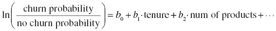
- Logistic regression. This is a powerful and well-established statistical algorithm that estimates the probabilities of the target classes. It is analogous to simple linear regression but for categorical outcomes. Logistic regression results have the form of continuous functions that estimate membership probabilities of the target classes:

where pj = probability of the target class j, pk probability of the reference target class k, Xi the predictors, bi the regression coefficients, and b0 the intercept of the model. The regression coefficients represent the effect of predictors.
For example, in the case of a binary target denoting churn,
In order to yield optimal results, it may require special data preparation, including potential screening and transformation (optimal binning) of the predictors. It demands some statistical experience yet, provided it is built properly, it can produce stable and understandable results.
- Neural networks. Neural networks are powerful machine-learning algorithms that use complex, nonlinear mapping functions for estimation and classification. They consist of neurons organized in layers. The input layer contains the predictors or input neurons. The output layer includes the target field. These models estimate weights that connect predictors (input layer) to the output. Models with more complex topologies may also include intermediate, hidden layers, and neurons. The training procedure is an iterative process. Input records, with known outcome, are presented to the network, and model prediction is evaluated in respect to the observed results. Observed errors are used to adjust and optimize the initial weight estimates. They are considered as opaque or “black box” solutions since they do not provide an explanation of their predictions. They only provide a sensitivity analysis, which summarizes the predictive importance of the input fields. They require minimum statistical knowledge but, depending on the problem, may require long processing times for training.
- Support Vector Machine (SVM). SVM is a classification algorithm that can model highly nonlinear complex data patterns and avoid overfitting, that is, the situation in which a model memorizes patterns only relevant to the specific cases analyzed. SVM works by mapping data to a high-dimensional feature space in which records become more easily separable (i.e., separated by linear functions) in respect to the target categories. Input training data are appropriately transformed through nonlinear kernel functions, and this transformation is followed by a search for simpler functions, that is, linear functions, which optimally separate cases. Analysts typically experiment with different kernel functions and compare the results. Overall, SVM is an effective yet demanding algorithm, in terms of processing time and resources. Additionally, it lacks transparency since the predictions are not explained, and only the importance of predictors is summarized.
- Bayesian networks. Bayesian networks are statistical models based on the Bayes theorem. They are probabilistic models as they estimate the probabilities of belonging to each target class. Bayesian belief networks, in particular, are graphical models which provide a visual representation of the attribute relationships, ensuring transparency and explanation of the model rationale.
1.3.1.2 Estimation (regression) models
Estimation models, also referred to as regression models, deal with continuous numeric outcomes. By using linear or nonlinear functions, they use the input fields to estimate the unknown values of a continuous target field.
Estimation algorithms can be used to predict attributes like the following:
- The expected balance of the savings accounts of the customers of a bank in the near future
- The estimated loss given default (LGD) incurred after a customer has defaulted
- The expected revenue from a customer within a specified time period
A dataset with historical data and known values of the continuous output is required for the model training. A mapping function is then identified that associates the available inputs to the output values. These models are also referred to as regression models, after the well-known and established statistical algorithm of ordinary least squares regression (OLSR). The OLSR estimates the line that best fits the data and minimizes the observed errors, the so-called least squares line. It requires some statistical experience, and since it is sensitive to possible violations of its assumptions, it may require specific data examination and processing before building. The final model has the intuitive form of a linear function with coefficients denoting the effect of predictors to the outcome. Although transparent, it has inherent limitations that may affect its performance in complex situations of nonlinear relationships and interactions between predictors.
Nowadays, traditional regression is not the only available estimation algorithm. New techniques, with less stringent assumptions, which also capture nonlinear relationships, can also be employed to handle continuous outcomes. More specifically, polynomial regression, neural networks, SVM, and regression trees such as CART can also be employed for the prediction of continuous attributes.
1.3.1.3 Feature selection (field screening)
The feature selection (field screening) process is a preparation step for the development of classification and estimation (regression) models. The situation of having hundreds of candidate predictors is not an unusual case in complicated data mining tasks. Some of these fields though may not have an influence to the output that we want to predict.
The basic idea of feature selection is to use basic statistical measures to assess and quantify the relationship of the inputs to the output. More specifically, feature selection is used to:
- Assess all the available inputs and rank them according to their association with the outcome.
- Identify the key predictors, the most relevant features for classification or regression.
- Screen the predictors with marginal importance, reducing the set of inputs to those related to the target field.
Some predictive algorithms, including Decision Trees, integrate screening mechanisms that internally filter out the unrelated predictors. A preprocessing feature selection step is also available in Data Mining for Excel, and it can be invoked when building a predictive model. Feature selection can efficiently reduce data dimensionality, retaining only a subset of significant inputs so that the training time is reduced with no or insignificant loss of accuracy.
1.3.2 Unsupervised models
In unsupervised modeling, only input fields are involved. The scope is the identification of groupings and associations. Unsupervised models include:
- Cluster models
In cluster models, the groups are not known in advance. Instead, the algorithms analyze the input data patterns and identify the natural groupings of instances/cases. When new cases are scored by the generated cluster model, they are assigned into one of the revealed clusters.
-
Association (affinity) and sequence models
Association and sequence models also belong to the class of unsupervised algorithms. Association models do not involve direct prediction of a single field. In fact, all fields have a double role, since they act as inputs and outputs at the same time. Association algorithms detect associations between discrete events, products, and attributes. Sequence algorithms detect associations over time.
- Dimensionality reduction models
Dimensionality reduction algorithms “group” fields into new compound measures and reduce the dimensions of data without sacrificing much of the information of the original fields.
1.3.2.1 Cluster models
Cluster models automatically detect the underlying groups of cases, the clusters. The clusters are not known in advance. They are revealed by analyzing the observed input data patterns. Clustering algorithms assess the similarity of the records/customers in respect to the clustering fields, and they assign them to the revealed clusters accordingly. Their goal is to detect groups with internal homogeneity and interclass heterogeneity.
Clustering algorithms are quite popular, and their use is widespread from data mining to market research. They can support the development of different segmentation schemes according to the clustering attributes used: behavioral, attitudinal, or demographical segmentation.
The major advantage of the clustering algorithms is that they can efficiently manage a large number of attributes and create data-driven segments. The revealed segments are not based on personal concepts, intuitions, and perceptions of the business people. They are induced by the observed data patterns, and provided they are properly built, they can lead to results with real business meaning and value. Clustering models can analyze complex input data patterns and suggest solutions that would not otherwise be apparent. They reveal customer typologies, enabling tailored marketing strategies.
Nowadays, various clustering algorithms are available which differ in their approach for assessing the similarity of the cases. According to the way they work and their outputs, the clustering algorithms can be categorized in two classes, the hard and the soft clustering algorithms. The hard clustering algorithms assess the distances (dissimilarities) of the instances. The revealed clusters do not overlap and each case is assigned to a single cluster.
Hard clustering algorithms include:
- Agglomerative or hierarchical. In a way, it is the “mother” of all clustering algorithms. It is called hierarchical or agglomerative since it starts by a solution where each record comprises a cluster and gradually groups records up to the point where all records fall into one supercluster. In each step, it calculates the distances between all pairs of records and groups the ones most similar. A table (agglomeration schedule) or a graph (dendrogram) summarizes the grouping steps and the respective distances. The analyst should then consult this information, identify the point where the algorithm starts to group disjoint cases, and then decide on the number of clusters to retain. This algorithm cannot effectively handle more than a few thousand cases. Thus, it cannot be directly applied in most business clustering tasks. A usual workaround is to a use it on a sample of the clustering population. However, with numerous other efficient algorithms that can easily handle even millions of records, clustering through sampling is not considered an ideal approach.
- K-means. K-means is an efficient and perhaps the fastest clustering algorithm that can handle both long (many records) and wide datasets (many data dimensions and input fields). In K-means, each cluster is represented by its centroid, the central point defined by the averages of the inputs. K-means is an iterative, distance-based clustering algorithm in which cases are assigned to the “nearest” cluster. Unlike hierarchical, it does not need to calculate distances between all pairs of records. The number of clusters to be formed is predetermined and specified by the user in advance. Thus, usually a number of different solutions should be tried and evaluated before approving the most appropriate. It best handles continuous clustering fields.
- K-medoids. K-medoids is a K-means variant which differs from K-means in the way clusters are represented during the model training phase. In K-means, each cluster is represented by the averages of inputs. In K-medoids, each cluster is represented by an actual, representative data point instead of using the hypothetical point defined by the cluster means. This makes this algorithm less sensitive to outliers.
- TwoStep cluster. A scalable and efficient clustering model, based on the BIRCH algorithm, included in IBM SPSS Modeler. As the name implies, it processes records in two steps. The first step of preclustering makes a single pass of the data, and records are assigned to a limited set of initial subclusters. In the second step, initial subclusters are further grouped, into the final segments.
- Kohonen Network/Self-Organizing Map (SOM). Kohonen Networks are based on neural networks, and they typically produce a two-dimensional grid or map of the clusters, hence the name SOM. Kohonen Networks usually take longer time to train than K-means and TwoStep, but they provide a different and worth trying view on clustering.
The soft clustering techniques on the other end use probabilistic measures to assign the cases to clusters with a certain probabilities. The clusters can overlap and the instances can belong to more than one cluster with certain, estimated probabilities. The most popular probabilistic clustering algorithm is Expectation Maximization (EM) clustering.
1.3.2.2 Association (affinity) and sequence models
Association models analyze past co-occurrences of events and detect associations and frequent itemsets. They associate a particular outcome category with a set of conditions. They are typically used to identify purchase patterns and groups of products often purchased together.
Association algorithms generate rules of the following general format:
- IF (ANTECEDENTS) THEN CONSEQUENT
For example:
- IF (product A and product C and product E and…) THEN product B
More specifically, a rule referring to supermarket purchases might be:
- IF EGGS & MILK & FRESH FRUIT THEN VEGETABLES
This simple rule, derived by analyzing past shopping carts, identifies associated products that tend to be purchased together: when eggs, milk, and fresh fruit are bought, then there is an increased probability of also buying vegetables. This probability, referred to as the rule’s confidence, denotes the rule’s strength.
The left or the IF part of the rule consists of the antecedents or conditions: a situation that when holds true, the rule applies and the consequent shows increased occurrence rates. In other words, the antecedent part contains the product combinations that usually lead to some other product. The right part of the rule is the consequent or the conclusion: what tends to be true when the antecedents hold true. The rule complexity depends on the number of antecedents linked with the consequent.
These models aim at:
- Providing insight on product affinities. Understand which products are commonly purchased together. This, for instance, can provide valuable information for advertising, for effectively reorganizing shelves or catalogues and for developing special offers for bundles of products or services.
- Providing product suggestions. Association rules can act as a recommendation engine. They can analyze shopping carts and help in direct marketing activities by producing personalized product suggestions, according to the customer’s recorded behavior.
This type of analysis is referred to as market basket analysis since it originated from point-of-sale data and the need of understanding consuming shopping patterns. Its application was extended though to also cover any other “basketlike” problem from various other industries. For example:
- In banking, it can be used for finding common product combinations owned by customers.
- In telecommunications, for revealing the services that usually go together.
- In web analytics, for finding web pages accessed in single visits.
Association models are unsupervised since they do not involve a single output field to be predicted. They analyze product affinity tables: multiple fields that denote product/service possession. These fields are at the same time considered as inputs and outputs. Thus, all products are predicted and act as predictors for the rest of the products.
Usually, all the extracted rules are described and evaluated in respect to three main measures:
- The support: it assesses the rule’s coverage or “how many records constitute the rule.” It denotes the percentage of records that match the antecedents.
- The confidence: it assesses the strength and the predictive ability of the rule. It indicates “how likely is the consequent, given the antecedents.” It denotes the consequent percentage or probability, within the records that match the antecedents.
- The lift: it assesses the improvement of the predictive ability when using the derived rule compared to randomness. It is defined as the ratio of the rule confidence to the prior confidence of the consequent. The prior confidence is the overall percentage of the consequent within all the analyzed records.
The Apriori and the FP-growth algorithms are popular association algorithms.
Sequence algorithms analyze paths of events in order to detect common sequences. They are used to identify associations of events/purchases/attributes over time. They take into account the order of events and detect sequential associations that lead to specific outcomes. Sequence algorithms generate rules analogous to association algorithms with one difference: a sequence of antecedent events is strongly associated with the occurrence of a consequent. In other words, when certain things happen with a specific order, a specific event has increased probability to follow. Their general format is:
- IF (ANTECEDENTS with a specific order) THEN CONSEQUENT
Or, for example, a rule referring to bank products might be:
- IF SAVINGS & THEN CREDIT CARD & THEN SHORT TERM DEPOSIT THEN STOCKS
This rule states that bank customers who start their relationship with the bank as savings customers and subsequently acquire a credit card and a short-term deposit present increased likelihood to invest in stocks. The support and confidence measures are also applicable in sequence models.
The origin of sequence modeling lies in web mining and click stream analysis of web pages; it started as a way to analyze web log data in order to understand the navigation patterns in web sites and identify the browsing trails that end up in specific pages, for instance, purchase checkout pages. The use of these algorithms has been extended, and nowadays, they can be applied to all “sequence” business problems. They can be used as a mean for predicting the next expected “move” of the customers or the next phase in a customer’s life cycle. In banking, they can be applied to identify a series of events or customer interactions that may be associated with discontinuing the use of a product; in telecommunications, to identify typical purchase paths that are highly associated with the purchase of a particular add-on service; and in manufacturing and quality control, to uncover signs in the production process that lead to defective products.
1.3.2.3 Dimensionality reduction models
As their name implies, dimensionality reduction models aim at effectively reducing the data dimensions and remove the redundant information. They identify the latent data dimensions and replace the initial set of inputs with a core set of compound measures which simplify subsequent modeling while retaining most of the information of the original attributes.
Factor, Principal Components Analysis (PCA), and Independent Component Analysis (ICA) are among the most popular data reduction algorithms. They are unsupervised, statistical algorithms which analyze and substitute a set of continuous inputs with representative compound measures of lower dimensionality.
Simplicity is the key benefit of data reduction techniques, since they drastically reduce the number of fields under study to a core set of composite measures. Some data mining techniques may run too slow or may fail to run if they have to handle a large number of inputs. Situations like these can be avoided by using the derived component scores instead of the original fields.
1.3.2.4 Record screening models
Record screening models are applied for anomaly or outlier detection. They try to identify records with odd data patterns that do not “conform” to the typical patterns of the “normal” cases.
Unsupervised record screening models can be used for:
- Data auditing, as a preparation step before applying subsequent data mining models
- Fraud discovery
Valuable information is not only hidden in general data patterns. Sometimes rare or unexpected data patterns can reveal situations that merit special attention or require immediate actions. For instance, in the insurance industry, unusual claim profiles may indicate fraudulent cases. Similarly, odd money transfer transactions may suggest money laundering. Credit card transactions that do not fit the general usage profile of the owner may also indicate signs of suspicious activity.
Record screening algorithms can provide valuable help in fraud discovery by identifying the “unexpected” data patterns and the “odd” cases. The unexpected cases are not always suspicious. They may just indicate an unusual yet acceptable behavior. For sure though, they require further investigation before being classified as suspicious or not.
Record screening models can also play another important role. They can be used as a data exploration tool before the development of another data mining model. Some models, especially those with a statistical origin, can be affected by the presence of abnormal cases which may lead to poor or biased solutions. It is always a good idea to identify these cases in advance and thoroughly examine them before deciding for their inclusion in subsequent analysis.
The examination of record distances as well as standard data mining techniques, such as clustering, can be applied for anomaly detection. Anomalous cases can often be found among cases distant from their “neighbors” or among cases that do not fit well in any of the emerged clusters or lie in sparsely populated clusters.
1.4 The data
The success of a data mining project strongly depends on the breadth and quality of the available data. That’s why the data preparation phase is typically the most time consuming phase of the project. Data mining applications should not be considered as one-off projects but rather as ongoing processes, integrated in the organization’s marketing strategy. Data mining has to be “operationalized.” Derived results should be made available to marketers to guide them in their everyday marketing activities. They should also be loaded in the organization’s frontline systems in order to enable “personalized” customer handling. This approach requires the setting up of well-organized data mining procedures, designed to serve specific business goals, instead of occasional attempts which just aim to cover sporadic needs.
In order to achieve this and become a “predictive enterprise,” an organization should focus on the data to be mined. Since the goal is to turn data into actionable knowledge, a vital step in this “mining quest” is to build the appropriate data infrastructure. Ad hoc data extraction and queries which just provide answers to a particular business problem may soon end up into a huge mess of unstructured information. The proposed approach is to design and build a central mining datamart that will serve as the main data repository for the majority of the data mining applications.
1.4.1 The mining datamart
All relevant information should be taken into account in the datamart design. Useful information from all available data sources, including internal sources such as transactional, billing and operational systems, and external sources such as market surveys and third-party lists, should be collected and consolidated in the datamart framework. After all, this is the main idea of the datamart: to combine all important blocks of information in a central repository that can enable the organization to have a complete a view of each customer.
The mining data mart should:
- Integrate data from all relevant sources.
- Provide a complete view of the customer by including all attributes that characterize each customer and his/hers relationship with the organization.
- Contain preprocessed information, summarized at the minimum level of interest, for instance, at an account or at a customer level. To facilitate data preparation for mining purposes, preliminary aggregations and calculations should be integrated in the loading of the datamart.
- Be updated on a regular and frequent basis to contain the current view of the customer.
- Cover a sufficient time period (enough days or months, depending on the specific situation) so that the relevant data can reveal stable and nonvolatile behavioral patterns.
- Contain current and historical data so that the view of the customer can be examined in different points in time. This is necessary since in many data mining projects and in classification models in particular, analysts have to associate behaviors of a past observation period with events occurring in a subsequent outcome period.
- Cover the requirements of the majority of the upcoming mining tasks, without the need of additional implementations and interventions from the IT.
1.4.2 The required data per industry
Table 1.3 presents an indicative, minimum list of required information that should be loaded and available in the mining datamart of retail banking.
Table 1.3 The minimum required data for the mining datamart of retail banking
| Product mix and product utilization: ownership and balances | |
| Product ownership and balances per product groups/subgroups For example:
|
|
| Frequency (number) and volume (amount) of transactions | |
| Transactions by transaction type For example:
|
Transactions by transaction channel For example:
|
| Product (account) openings/terminations | |
| For the specific case of credit cards, frequency and volume of purchases by type (one-off, installments, etc.), and merchant category | |
| Credit score and arrears history | |
| Information on the profitability of customers | |
| Customer status history (active, inactive, dormant, etc.) and core segment membership (retail, corporate, private banking, affluent, mass, etc.) | |
| Registration and sociodemographical information of customers | |
Table 1.4 lists the minimum blocks of information that should reside in the datamart of a mobile telephony operator (for residential customers).
Table 1.4 The minimum required data for the mining datamart of mobile telephony (residential customers)
| Phone usage: number of calls/minutes of calls/traffic | |||
Usage by call direction and network type
|
Usage by core service type For example:
|
Usage by origination/destination operator For example:
|
Usage by call day/time For example:
|
| Customer communities: distinct telephone numbers with calls from or to | |||
| Information by call direction (incoming/outgoing) and operator (on-net/mobile telephony competitor operator/fixed telephony operator) | |||
| Top-up history (for prepaid customers), frequency, value, and recency of top-ups | |||
| Information by top-up type | |||
| Rate plan history (opening, closings, migrations) | |||
| Billing, payment, and credit history (average number of days till payment, number of times in arrears, average time remaining in arrears, etc.) | |||
| Financial information such as profit and cost for each customer (ARPU, MARPU) | |||
| Status history (active, suspended, etc.) and core segmentation information (consumer postpaid/contractual, consumer prepaid customers) | |||
| Registration and sociodemographical information of customers | |||
Table 1.5 lists the minimum information blocks that should be loaded in the datamart of retailers.
Table 1.5 The minimum required data for the mining datamart of retailers
| RFM attributes: recency, frequency, monetary overall, and per product category | |||
| Time since the last transaction (purchase event) or since the most recent visit day Frequency (number) of transactions or number of days with purchases Value of total purchases | |||
| Spending: purchases amount and number of visits/transactions | |||
| Relative spending by product hierarchy and private labels For example:
|
Relative spending by store/department For example:
|
Relative spending by date/time
|
Relative spending by channel of purchase For example:
|
| Usage of vouchers and reward points | |||
| Payments by type (e.g., cash, credit card) | |||
| Registration data collected during the loyalty scheme application process | |||
1.4.3 The customer “signature”: from the mining datamart to the enriched, marketing reference table
Most data mining applications require a one-dimensional, flat table, typically at a customer level. A recommended approach is to consolidate the mining datamart information, often spread in a set of database tables, into one table which should be designed to cover the key mining as well as marketing and reporting needs. This table, also referred to as the marketing reference table, should integrate all the important customer information, including demographics, usage, and revenue data, providing a customer “signature”: a unified view of the customer. Through extensive data processing, the data retrieved from the datamart should be enriched with derived attributes and informative KPIs to summarize all the aspects of the customer’s relationship with the organization.
The reference table typically includes data at a customer level, though the data model of the mart should support the creation of custom reference tables of different granularities. It should be updated at a regular basis to provide the most recent view of each customer, and it should be stored to track the customer view over time. The key idea is to comprise a good starting point for the fast creation of a modeling file for all the key future analytical applications.
Typical data management operations required to construct and maintain the marketing reference tables include:
- Filtering of records. Filtering of records based on logical conditions to include only records of interest.
- Joins. Consolidation of information of different data sources using key fields to construct a total view of each customer.
- Aggregations/group by. Aggregation of records to the desired granularity. Replacement of the input records with summarized output records, based on statistical functions such as sums, means, count, minimum, and maximum.
- Restructure/pivoting. Rearrangement of the original table with the creation of multiple separate fields. Multiple records, for instance, denoting credit card purchases by merchant type, can be consolidated into a single record per customer, summarized with distinct purchase fields per merchant type.
- Derive. Construction of new, more informative fields which better summarize the customer behavior, using operators and functions on the existing fields.
The derived measures in the marketing reference table should include:
- Sums/averages. Behavioral fields are summed or averaged to summarize usage patterns over a specific time period. For instance, a set of fields denoting the monthly average number of transactions by transaction channel (ATM, Internet, phone, etc.) or by transaction type (deposit, withdrawal, etc.) can reveal the transactional profile of each customer. Sums and particularly (monthly) averages take into account the whole time period examined and not only the most recent past, ensuring the capture of stable, nonvolatile behavioral patterns.
- Ratios. Ratios (proportions) can be used to denote the relative preference/importance of usage behaviors. As an example, let’s consider the relative ratio (the percentage) of the total volume of transactions per transaction channel. These percentages reveal the channel preferences while also adjust for the total volume of transactions of each customer. Other examples of this type of measures include the relative usage of each call service type (voice, SMS, MMS, etc.) in telecommunications or the relative ratio of assets versus lending balances in banking. Apart from ratios, plain numeric differences can also be used to compare usage patterns.
- Flags. Flag fields are binary (dichotomous) fields that directly and explicitly record the occurrence of an event of interest or the existence of an important usage pattern. For instance, a flag field might show whether a bank customer has made any transactions through an alternative channel (phone, Internet, SMS, etc.) in the period examined or whether a telecommunications customer has used a service of particular interest.
- Deltas. Deltas capture changes in the customer’s behavior over time. They are especially useful for supervised (predictive) modeling since a change in behavior in the observation period may signify the occurrence of an event such as churn, default, etc. in the outcome period. Deltas can include changes per month, per quarter, or per year of behavior. As an example, let’s consider the monthly average amount of transactions. The ratio of this average over the last 3 months to the total average over the whole period examined is a delta measure which shows whether the transactional volume has changed during the most recent period.
1.5 Summary
In this chapter, we’ve presented a brief overview of the main concepts of data mining. We’ve outlined how can data mining help an organization to better address the CRM objectives and achieve “individualized” and more effective customer management through customer insight. We’ve introduced the main types of data mining models and algorithms and a process model, a methodological framework for designing and implementing successful data mining projects. We’ve also presented the importance of the mining datamart and provided indicative lists of required information per industry.
Chapters 2 and 3 are dedicated in the detailed explanation of the methodological steps for classification and segmentation modeling. After clarifying the roadmap, we describe the tools, the algorithms. Chapters 4 and 5 explain in plain words some of the most popular and powerful data mining algorithms for classification and clustering. The second part of the book is the “hands-on” part. The knowledge of the previous chapters is applied in real-world applications of various industries using three different data mining tools. A worth noting lesson that I’ve learned after concluding my journey in this book is that it is not the tool that matters the most but the roadmap. Once you have an unambiguous business and data mining goal and a clear methodological approach, then you’ll most likely reach your target, yielding comparable results, regardless of the data mining software used.