Chapter 3
Probabilistic Indicators for the Assessment of Reliability and Security of Future Power Systems
Bart W. Tuinema1, Nikoleta Kandalepa2 and José Luis Rueda-Torres3
1Researcher of Intelligent Electrical Power Grids, Department of Electrical Sustainable Energy, Delft University of Technology, The Netherlands
2Grid Strategist, Asset Management, TenneT TSO B.V., Arnhem, The Netherlands
3Assistant professor of Intelligent Electrical Power Grids, Department of Electrical Sustainable Energy, Delft University of Technology, The Netherlands
3.1 Introduction
Current developments in the power system put increasing stresses on the transmission network. The transition towards a renewable energy supply, the integration of large-scale renewable energy sources (RES) and the liberalisation of the electricity market are some of the challenges for the transmission network. At the same time, the lowest cost of an ageing transmission network is strived for. To prevent large blackouts, reliability analysis and reliability management are of the utmost importance. While deterministic approaches and criteria have been used effectively in the past, probabilistic methods will be increasingly applied in the future as these provide more insight into the reliability of the transmission network.
This chapter describes how probabilistic reliability analysis is used to study the reliability of large transmission networks. We discuss how probabilistic reliability analysis is related to deterministic criteria and risk categories. Two common approaches for probabilistic reliability analysis will be presented, that is, state enumeration and Monte Carlo simulation. In a case study of the Dutch extra-high voltage (EHV) transmission network, these methods are applied to analyse the reliability impact of EHV underground cables.
The organisation of this chapter is as follows. In Section 3.2, the concept of time horizons in the planning and operation of a power system is introduced. Several reliability indicators that are commonly used in probabilistic reliability analysis are discussed in Section 3.3. In Section 3.4, two methods for reliability analysis are described: state enumeration and Monte Carlo simulation. Section 3.5 describes a case study of the Dutch transmission network. General conclusions are discussed in Section 3.6.
3.2 Time Horizons in the Planning and Operation of Power Systems
3.2.1 Time Horizons
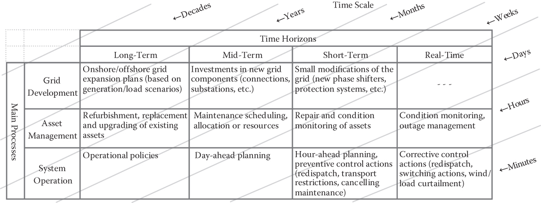
In the planning and operation of power systems, Transmission System Operator (TSO) actions are performed in different processes and time horizons [1]. The main objective is to maintain a high level of reliability. Basically, three main processes can be distinguished: grid development, asset management and system operation. TSO actions are taken in time horizons ranging from long-term, mid-term and short-term to real-time. Table 3.1 shows some typical activities for each of the main TSO processes and for different time horizons. As can be seen, TSO actions range from long-term grid development (with a timescale of decades) to real-time system operation (with a timescale up to real-time).
Table 3.1 Actions taken during different time horizons [1]
 |
3.2.2 Overlapping and Interaction
There is always some overlap between the three main TSO processes. For example, the installation of new assets can be a grid development activity or an asset management activity. In asset management, maintenance activities are scheduled, but these could be cancelled in system operation during critical situations. Traditionally, TSO activities were mostly performed sequentially, as shown in Figure 3.1. An example is the Dutch 380 kV-ring, which was designed to be n-2 redundant (n-1 redundant during maintenance). This gave enough room to plan maintenance activities in asset management while still providing n-1 redundancy during system operation. As can be seen in Figure 3.1, in the sequential approach there is only a small overlap between the TSO processes.
In the future, the developments as mentioned in the introduction of this chapter are expected to put more stress on the transmission network. The transmission network will become more heavily loaded, and the room to plan TSO activities will decrease. Consequently, the overlap between the processes will increase and the planning of TSO activities will be more interacted, as illustrated in Figure 3.1. A typical example is the development of offshore grids. Other studies showed that it is often not economical to apply full n-1 redundancy in offshore networks. However, if there is no redundancy, maintenance activities will have more consequences for the availability of the offshore grid and therefore maintenance planning can become challenging. Moreover, without offshore redundancy, failures of offshore networks can have a large impact on the onshore power system during system operation as it becomes more likely that a substantial amount of wind capacity is interrupted. Here, the interaction of grid development (n-1 redundancy), asset management (maintenance planning) and operational planning (remedial actions) can be clearly seen.
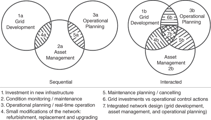
Figure 3.1 Interactions among three TSO processes [1].
3.2.3 Remedial Actions
As there is always interaction and overlap between the three main TSO processes, it is important to model this in the reliability analysis as well. In the application example described in this chapter, the focus is on long-term grid development decisions and the consequences for (short-term and real-time) system operation. It will be discussed how the application of new underground cable connections in grid development is related to remedial actions like generation redispatch and load curtailment in system operation.
Remedial actions are operational interventions performed by the TSO to avoid/relieve overload of the network during critical situations. Typical remedial actions are: application of PSTs (Phase-Shifting Transformers), network reconfiguration, cancelling maintenance, local generation redispatch, cross-border-redispatch and load/wind curtailment [2]. With PSTs, the phase shift of the voltage can be varied such that the magnitude and direction of the power flow can be controlled. The network can be reconfigured by performing switching actions to reduce the loading of overloaded connections. This is mainly applied in the high voltage (HV) and lower voltage networks. If a connection is under maintenance in an overloaded part of the network, it can be decided to cancel this maintenance to relieve the loading of other connections. By performing local (or national) generator redispatch, the production of some generators is increased while it is decreased for other generators to reduce the loading of connections in overloaded parts of the network. If local generator redispatch is not sufficient, cross-border (or international) redispatch can be performed. Wind curtailment can also be used to relieve the overloading of the network. The last resort to relieve overloading is to disconnect load by load curtailment (or load shedding).
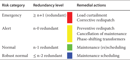
In system operation, a risk framework is often used in which the current risk status of the network is indicated. The reliability (measured as the level of redundancy) can be related to the risk categories of this risk framework [3]. Remedial actions can be related to these risk categories as well. Table 3.2 shows that remedial actions like PSTs and maintenance cancellation are often applied first, while load curtailment is the last resort. Although Table 3.2 shows how remedial actions are related to the risk categories and redundancy levels, the choice for a certain remedial action always depends on the situation.
Table 3.2 Risk categories, redundancy levels and remedial actions
 |
3.3 Reliability Indicators
3.3.1 Security-of-Supply Related Indicators
The main function of a power system is to supply the load. If the power system is not able to supply its load, it is considered as unreliable. Therefore, the reliability indicator security-of-supply is often regarded as the most important Key Performance Indicator (KPI) of power system reliability. Several reliability indicators exist that are directly related to security-of-supply. Some reliability indicators are specially defined to measure the reliability of a part of the power system, while others are developed for combined generation/ transmission/distribution systems.
Reliability indicators developed to measure the reliability of the generation system [4, 5]:
- LOLP (Loss of Load Probability): probability that the demanded power cannot be supplied (partially or completely) by the generation system. The LOLP is often determined based on a per-hour study for a studied time period (usually a year)
3.1
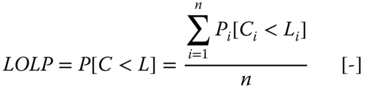
where:
- P[C<L]
- = probability that the generation capacity is smaller than the load [-]
- Pi[Ci<Li]
- = probability that the gen. capacity is smaller than the load for hour i [-]
- C
- = total available generation capacity [MW]
- Ci
- = total available generation capacity for hour i [MW]
- L
- = total load level [MW]
- Li
- = total load level for hour i [MW]
- n
- = total time of the studied period (8760 h for a whole year) [h]
- LOLE (Loss of Load Expectation): expected amount of time per period that the demanded power cannot be supplied (partially or completely) by the generation system
3.2
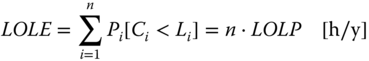
where:
- Pi[Ci<Li]
- = probability that the gen. capacity is smaller than the load for hour i [-]
- Ci
- = total available generation capacity for hour i [MW]
- Li
- = total load level for hour i [MW]
- n
- = total time of the studied period (8760 h/y for a whole year) [h/y]
- LOLP
- = loss of load probability [-]
- LOEE (Loss of Energy Expectation): total amount of energy that is expected not to be supplied during a given time period (usually on a yearly basis) because of failures of the generation system
3.3
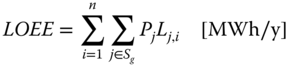
where:
- Pj
- = probability of generation capacity outage j [-]
- Lj
- = not delivered load because of capacity outage j [MW]
- n
- = total time of the studied period (8760 h/y for a whole year) [h/y]
- Sg
- = set of possible generation capacity outages
Other reliability indicators are developed to measure the reliability of combined (generation)/transmission/distribution networks [2, 4, 5]. A few of these are:
- PLC (Probability of Load Curtailment): probability that the demanded power cannot be supplied (partially or completely). The PLC is often determined based on a set of considered contingencies (single contingencies as well as higher-order contingencies) and a studied time period (usually on a yearly basis)
3.4
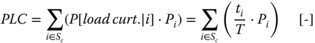
where:
- Sc
- = set of considered contingencies
- P[load curt.|i]
- = probability that contingency i causes load curtailment [-]
- Pi
- = probability of contingency i [-]
- ti
- = total time that there is load curtailment during the studied period,
- given that contingency i is present [h]
- T
- = total time of the studied period [h]
- EENS (Expected Energy Not Supplied): total amount of energy that is expected not to be supplied during a given time period (usually on a yearly basis) due to supply interruptions
3.5
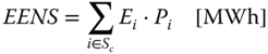
where:
- Sc
- = set of considered contingencies
- Ei
- = total curtailed energy in the study period if contingency i is present [MWh]
- Pi
- = probability of contingency i [-]
- SAIDI (System Average Interruption Duration Index): average outage duration of each customer during a given time period (usually on a yearly basis)
3.6
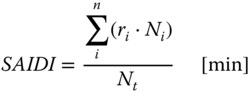
where:
- n
- = number of interruptions [-]
- ri
- = duration of interruption i [min]
- Ni
- = number of customers not served by interruption i [-]
- Nt
- = total number of customers [-]
- SAIFI (System Average Interruption Frequency Index): average number of interruptions per customer during a given time period (usually on yearly basis).
3.7
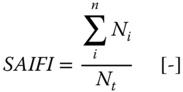
where:
- n
- = number of interruptions [-]
- Ni
- = number of customers not served by interruption i [-]
- Nt
- = total number of customers [-]
- CAIDI (Customer Average Interruption Duration Index): average interruption duration per interrupted customer during a given time period (usually on yearly basis)
3.8
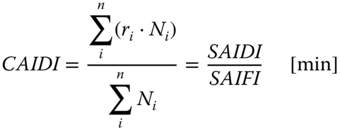
where:
- n
- = number of interruptions [-]
- ri
- = duration of interruption i [min]
- Ni
- = number of customers not served by interruption i [-]
3.3.2 Additional Indicators
Traditionally, power system reliability studies concentrate on these security-of-supply related indicators. Often, it is assumed that there is one TSO that can take any remedial action to secure the load supply. The liberalisation of the electricity market has, however, led to several new actors such as producers, consumers, service providers and system operators. All of these actors have their own vision on power system reliability. For example, consumers wish to have a reliable power supply, while producers wish to be connected to the grid and sell their electricity. For a TSO, the transmission network is reliable if the customers (i.e. producers and consumers) are able to trade in electricity, while the network should also be maintainable.
In this sense, the reliability of a power system is not only reflected by the security-of-supply, but also related to indicators like the probability of wind curtailment, the probability of generation redispatch and the maintenance possibilities. These aspects can be included in reliability analysis by calculating several reliability indicators instead of one. As remedial actions are related to the risk states (see Table 3.2), calculating the probability of these states can provide more insight as well. Possible additional reliability indicators are then [2]:
- Probability of Overload: probability that one or more connections in the network are overloaded during a given time period (usually on a yearly basis)
3.9
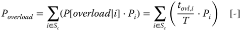
where:
- Sc
- = set of considered contingencies
- P[overload|i]
- = probability that contingency i causes an overloaded connection [-]
- Pi
- = probability of contingency i [-]
- tovl,i
- = total time that there is an overload during the studied period, given
- that contingency i is present [h]
- T
- = total time of the studied period [h]
- Probability of Generation Redispatch: probability that generation redispatch is applied during a given time period (usually on a yearly basis)
3.10
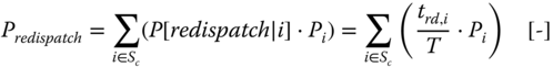
where:
- Sc
- = set of considered contingencies
- P[redispatch|i]
- = probability that contingency i causes generation redispatch [-]
- Pi
- = probability of contingency i [-]
- trd,i
- = total time that redispatch is applied during the studied period,
- given that contingency i is present [h]
- T
- = total time of the studied period [h]
- Expected Redispatch Costs: expected costs of the generation redispatch during a given time period (usually on a yearly basis)
3.11
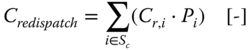
where:
- Sc
- = set of considered contingencies
- Cr,i
- = total redispatch costs during the study period, if contingency i is present [-]
- Pi
- = probability of contingency i [-]
- Probability of the Alert State: probability that the power system is in the alert state during a given time period (usually on a yearly basis)
3.12
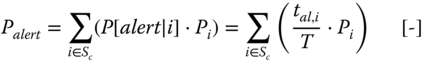
where:
- Sc
- = set of considered contingencies
- P[alert|i]
- = probability that contingency i leads to the alert state [-]
- Pi
- = probability of contingency i [-]
- tal,i
- = total time that the network is in the alert state during the studied
- period, given that contingency i is present [h]
- T
- = total time of the studied period [h]
The application example in Section 3.5 of this chapter will illustrate how a combination of reliability indicators provides more insight into the reliability of the power system.
3.4 Reliability Analysis
Based on various input information (such as load/generation scenarios and network parameters), the reliability of the transmission network can be calculated. Figure 3.2 shows an overview of this process. The different parts of the calculation process are discussed in the following sections.
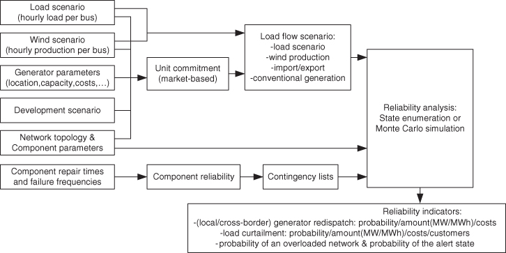
Figure 3.2 Overview of reliability analysis.
3.4.1 Input Information
The following input information is needed to perform the reliability analysis:
- Load scenario: In the load scenario, the load is specified for every hour of a study year. The load is aggregated per substation in the studied network. The load scenario is based on the expected development of (domestic and industrial) load and assumptions about the development of RES and conventional generation.
- Wind scenario: In the wind scenario, the production of large-scale (offshore) wind parks is specified per hour of the study year. The wind scenario is based on a time series of the wind speed, taking parameters like the size and location of the wind farms into account.
- Generator parameters: For all generators in the studied power system, information such as the location, fuel type, costs and capacity is needed. This information also takes into account developments such as the installation or closure of units. National generators are included, as well as some generators in surrounding countries.
- Development scenario: In the development scenario, assumptions are made about the development of RES and conventional generation (e.g. [12]). Also, assumptions can be made about preferences for the generator units (e.g. preference for fuel type or location).
- Network topology & component parameters: This information includes the network topology, as well as all required information to perform a load flow calculation (e.g. component impedances and admittances, component capacities).
- Component repair times and failure frequencies: This information is needed to calculate the reliability of network components. Failure frequencies and repair times can be obtained from databases of historical failures. If the volume of available failure statistics is too limited (e.g. for new component types), estimations of failure frequency and repair time can be made.
3.4.2 Pre-calculations
The input information is now pre-processed in order to be used in the reliability analysis. The following calculations/analyses are performed:
- Unit commitment: In this analysis, the production of the generator units is scheduled such that all the load in the power system is supplied. The load scenario, wind scenario and generator parameters are the input information to this analysis. Network information and the assumptions of the development scenario can be used as restrictions for the unit commitment. The result of the unit commitment study is a generation scenario for the national generators and an import/export scenario, which is based on the generators in the surrounding countries.
- Component reliability: The reliability behaviour of network components is described based on the failure frequencies and repair times of the components. This information is then collected in contingency lists, which contain the contingencies to be considered in reliability analysis together with their parameters (such as failure frequency, repair time, unavailability [4, 5], component status). Independent as well as dependent failures, in which one cause leads to a simultaneous failure of multiple components, can be included in the contingency lists too.
3.4.3 Reliability Analysis
Based on the input information and the results of the pre-calculations (i.e. the load flow scenario, the network information and the contingency lists), the reliability of the network can now be analysed. There are two main approaches to probabilistic power system reliability analysis: state enumeration and Monte Carlo simulation [4, 5]. The first is a structured analytical study of possible contingencies, the second is a computer simulation. Both approaches are discussed in this section.
- State enumeration: In state enumeration, the reliability analysis is based on the possible contingency states. The general algorithm for state enumeration is shown in Figure 3.3. It can be seen that for every contingency state, the probability of this contingency state is calculated and a load flow is performed. If there is an overload in the network, remedial actions are applied. From the application of these remedial actions, information is gathered that will be used to calculate the reliability indicators. After applying remedial actions, the load flow is calculated again and if there still is an overload, more (or other) remedial actions are applied. The state enumeration stops when all contingency states to be considered have been studied.
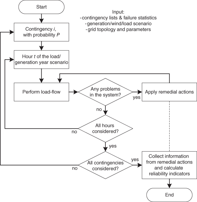
Figure 3.3 Algorithm for the reliability assessment using state enumeration.
- Monte Carlo simulation: In a Monte Carlo simulation, the reliability of the power system is studied by performing a computer simulation. The general algorithm of a Monte Carlo simulation is shown in Figure 3.4. The Monte Carlo simulation uses the same input information as the state enumeration, albeit in a somewhat different way. First, from the failure frequencies specified in the contingency lists, the first time to failure (TTF) is sampled assuming an exponential distribution [4, 5]. The component with the smallest TTF will fail first and using its repair time, the time at which this component will be repaired is calculated. Until the component is repaired, a contingency exists in the network and the load flow is calculated for this period using the generation/wind/export/load scenario. If there is an overload in the network, remedial actions are applied in a similar way to state enumeration. Also similarly to state enumeration, intermediate results are collected to calculate the reliability indicators. A somewhat more complicated situation exists when a second contingency occurs before the first contingency is repaired. In this case, there are multiple contingencies in the network, which can also be combinations of independent/dependent failures as specified in the contingency lists. This situation ends when one of the contingencies is repaired, after which the other contingency is still being repaired. In contrast to state enumeration, it is possible (but very unlikely) that higher-order failure combinations occur during the Monte Carlo simulation, because component failures are randomly sampled and multiple components can be sampled as ‘failed’. The simulation stops when the given simulation time is reached.
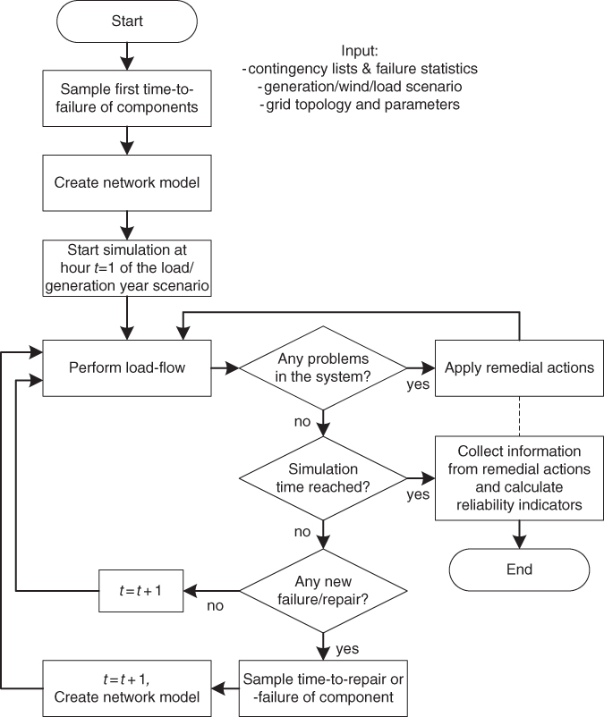
Figure 3.4 Algorithm for the reliability assessment using Monte Carlo simulation.
3.4.4 Output: Reliability Indicators
The results of the reliability analysis are various reliability indicators. As described in Section 3.3, these reliability indicators can be directly related to security-of-supply, but can also be additional reliability indicators. Together, these reliability indicators give a more complete understanding of the reliability of the studied transmission network.
3.5 Application Example: EHV Underground Cables
The reliability analysis as described in the previous section was applied to a case study of the Dutch extra-high voltage (EHV) transmission network. Currently, underground cables are installed in the backbone of the Dutch 380 kV network in the Randstad380 project [6]. So far, 380 kV Underground Cables (UGCs) have been installed in the Randstad380 South ring and another 380 kV cable project (Randstad380 North) is expected to come into operation in the near future. After the operation of both projects, around 20 kilometres will be underground in an entire route of approximately 80 km across the Randstad region. Figure 3.5 shows the Dutch EHV (380/220 kV) transmission network.
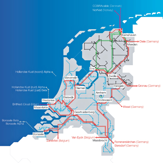
Figure 3.5 Dutch EHV transmission network (380/220 kV) [12].
As not much is known about the behaviour of EHV underground cables, various aspects like resonance behaviour, transient performance and reliability are being studied [7]–[10]. Regarding the reliability, previous research studied the reliability of cable components [7, 10] and the reliability of transmission links consisting of overhead lines and underground cables [9]. As underground cables will have an impact on the reliability of large transmission networks, the risk of further cabling of the EHV transmission network is also considered [2].
3.5.1 Input Parameters
The application example examines how the installation of more EHV underground cables (UGC) in the Dutch transmission grid affects the overall reliability level. Although the cable failure frequency is very close to that of overhead lines (OHL), the additional components of UGC (joints and terminations) reduce the reliability of the whole system [13]. Therefore, the unavailability of a connection is higher when it is partially or fully cabled than when it is completely an overhead line. Moreover, underground cables have a lower characteristic impedance. This is why it is important to study how the increased unavailability and the reduced impedance of the connection affect the overall reliability level.
As already described in Section 3.4, the reliability analysis consists of four major parts: contingency definition, load flow analysis, application of remedial actions if necessary and calculation of KPIs. A state enumeration is performed for the contingency types: independent single circuit failures, dependent double circuit failures, dependent triple circuit failures. All these contingencies refer to OHL and UGC failures. In addition, combinations of two of these contingency types are considered. In this way, 2nd-order contingencies can occur with two single circuit failures or with one double circuit failure and 6th-order contingencies are (only) reached by the combination of two triple circuit failures. Moreover, in this example three corrective actions are used with the following priority: national generator re-dispatch, cross-border re-dispatch and load curtailment. Taking these remedial actions into account, the state enumeration algorithm as shown in Figure 3.3 now becomes as shown in Figure 3.6.
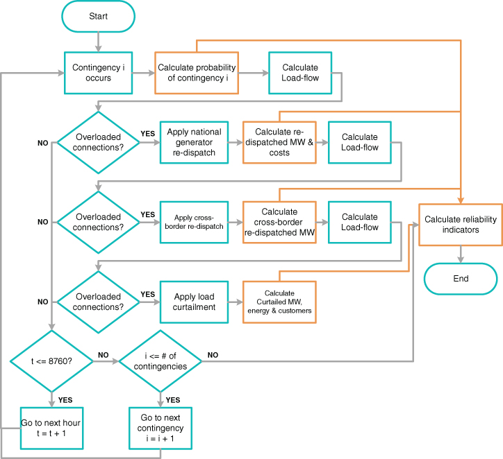
Figure 3.6 State enumeration-based algorithm for the case study [2].
In order to examine how further 380 kV cabling in the Dutch transmission network will impact the overall reliability level, simulations are performed by installing UGCs in three different connections (named Con1, Con2 and Con3). The PLC, the probability of overload and expected redispatch costs are calculated. The network topology and the required data are determined according to TenneT's scenario2020. It provides hourly data regarding generation (conventional/wind), load and export/import for the specific year. It is also important to describe the configuration of UGCs which is used in this study. As shown in Figure 3.7a, the UGCs consist of two circuits, and each circuit phase consists of two separate cables. In this configuration, a failure of a separate cable leads to a failure of one circuit, as operation with only one cable per circuit phase is undesirable in system operation.
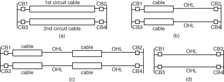
Figure 3.7 Configurations of underground cable connections.
In the case study, the cable length in the considered connections varies from 0% to 100% cabling with steps of 25%. The percentage refers to the transmission length of the connection and 0% means purely OHLs while 100% means a fully-cabled connection (as shown in Figure 3.7a). For example, in Figure 3.7b, 50% of the connection is cabled. The number of cable sections per connection can vary as well. For example, in Figure 3.7c there are two cable sections in the connection. Figure 3.7d shows the standard OHL connection configuration.
Due to the limited experience with EHV UGCs, there are no accurate values for their failure frequency and repair time. An earlier survey among European TSOs is used where a high and a low estimation of the failure frequencies are given, as shown in Tables 3.3 and 3.4 [7]. The repair time of UGCs is estimated as 730 h (1 month), which could be reduced to 336 h (2 weeks) if the repair process becomes more optimised in future [9]. For OHL, long experience has given more insight into failure statistics. The values are derived from actual failure statistics of the Dutch network [11].
Table 3.3 Failure frequency of EHV overhead lines and underground cables
| Failure frequency | ||
| OHL | 0.00220 [/cctkm·y] | |
| TSOs high | TSOs low | |
| Cable | 0.00120 [/cctkm·y] | 0.00079 [/cctkm·y] |
| Joint | 0.00035 [/comp·y] | 0.00016 [/comp·y] |
| Termination | 0.00168 [/comp·y] | 0.00092 [/comp·y] |
Table 3.4 Repair time of EHV overhead lines and underground cables
| Repair time | ||
| OHL | 8 h | |
| high | low | |
| UGC | 730 h | 336 h |
3.5.2 Results of Analysis
The reliability analysis algorithm developed (Figure 3.6) is used to execute a number of simulation sets, and both categories of KPIs (directly linked to loss of load and not directly linked to loss of load) are calculated. Fig. 3.8 shows how the PLC changes when varying cable length is installed in the three considered connections. While one of these connections includes UGCs, the others are full OHLs. There are three curves, each devoted to a specific connection. The y-axis represents the PLC in h/y, while in the x-axis the cable length is presented as percentage of the connection length. The point 0% indicates that the three connections are OHLs, and this is the starting point for all curves.
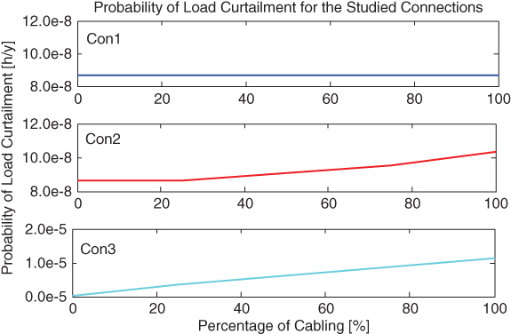
Figure 3.8 UGC in different connections – PLC.
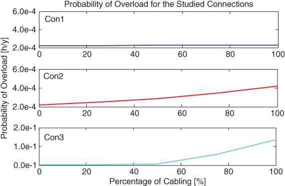
Figure 3.9 UGC in different connections – Probability of overload.
The installation of UGC in Con1 has no impact on the PLC, while the other two curves illustrate an upward trend as cable length increases. However, while 50% cabling in Con2 causes a 5% increase in PLC, the same percentage of cabling in Con3 leads to a 70 times higher probability. In order to explain this phenomenon, the relative loadings of these connections were studied, and it was observed that the maximum loadings present similar behaviour with the amount of increase of the indicator, namely very small loading for Con1, larger for Con2 and even more considerable for Con3. It seems that the loading of the connection where UGCs are installed influences the impact on the reliability level.
Fig. 3.9 examines the probability of overload when UGCs are installed in each of the three connections. By comparing Fig. 3.8 with Fig. 3.9, it can be seen that the probability of overload in Con1 shows a very small upward trend as cable length increases (and is not constant like the PLC). The other two connections are characterised by an increasing trend as well. It is also clear that the values of the probability of overload are orders of magnitude larger than those of the PLC.
Fig. 3.10 illustrates the expected redispatch costs when UGCs are installed in each of the three connections. By considering a specific percentage of cabling, the three points of the connections are depicted next to each other. This occurs for each cabling percentage. The diagram is normalised (logarithmic), where the base 1 represents the starting point (0% cabling, three connections as OHL). The expected redispatch costs confirm the remarks made so far. They show a growing trend with rising cable length, and the installation of UGCs in Con3 seems the most expensive option (from redispatch costs point of view). Con3 is a heavily-loaded connection, and its failure appears several times in the contingencies which lead to generator redispatch. On the other hand, Con1 appears to be the most economical solution, since even at 100% cabling, the increase of the indicator is less than 10% from the starting point.
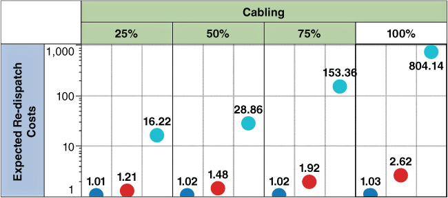
Figure 3.10 UGC in different connections – Expected redispatch costs. The leftmost point corresponds with Con1, the middle point corresponds with Con2, and the rightmost point corresponds with Con3.
The results were verified using a Monte Carlo simulation as shown in Figure 3.11.
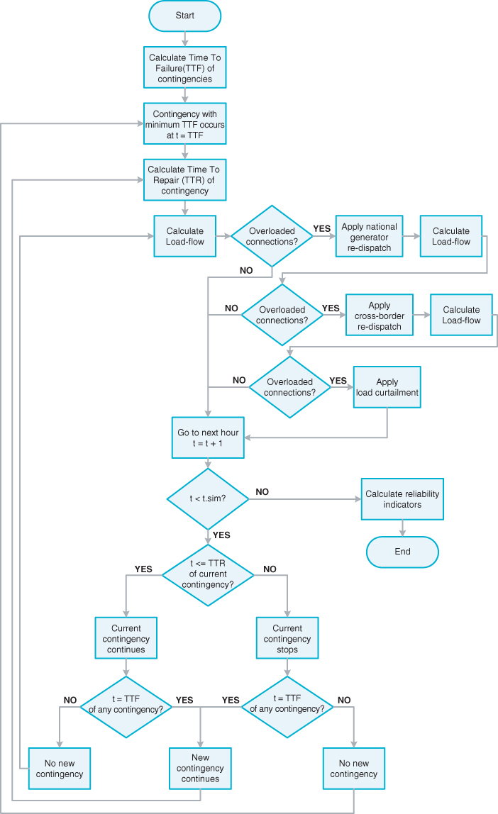
Figure 3.11 Monte Carlo simulation-based algorithm for the case study [2].
To sum up, the installation of UGC in specific connections might not influence the reliability indicators related to load curtailment, compared to the starting point. However, this does not mean that the level of reliability remains the same. It was shown in the results that in these cases, the reliability indicators which are not directly related to security-of-supply might demonstrate significant change leading to a lower reliability level. Therefore, it can be concluded that indicators not directly linked to load curtailment should be used as well.
3.6 Conclusions
This chapter discussed the probabilistic reliability analysis of transmission networks. It described how the planning and operation of power systems will change in future and what challenges can be expected. The most common probabilistic reliability indicators were presented and we discussed how these are related to deterministic criteria and risk categories and how these indicators can provide more insight into the reliability of power systems. The two probabilistic reliability analysis approaches, state enumeration and Monte Carlo simulation, were explained. In a case study of the Dutch EHV transmission network, these approaches were applied to study the reliability impact of EHV underground cables.
The case study clearly showed that multiple reliability indicators provide more insight into the reliability of the transmission network than one single reliability indicator. In some cases, a reliability indicator such as the Probability of Load Curtailment does not show any difference whereas other reliability indicators such as the probability of redispatch can show a difference. For a TSO, both load curtailment and generation redispatch can be risks in the liberalised electricity market. Decisions on future developments, such as the installation of underground cables in the EHV transmission network, should be based on a combination of reliability indicators as presented in this chapter.
For future work, it is of interest to study further on how the results of probabilistic reliability analysis must be interpreted. Also, the development of fast probabilistic reliability analysis and decision making would be beneficial, such that probabilistic reliability analysis can effectively be applied in system operation as well. Clear and intuitive deterministic criteria have been used for a long time; it should be studied how probabilistic reliability analysis can best complement deterministic criteria and approaches.
References
- 1 S.R. Khuntia, B.W. Tuinema, J.L. Rueda, M.A.M.M. van der Meijden, “Time-horizons in the planning and operation of transmission networks: an overview”, IET Generation, Transmission & Distribution, Vol. 10, No. 4, Oct. 2016, pp 841–848.
- 2 N. Kandalepa, Reliability Modeling in Transmission Networks – An explanatory Study for further EHV underground Cabling in the Netherlands, MSc Thesis, Delft University of Technology, Delft, the Netherlands, 2015. Available online: repository.tudelft.nl.
- 3 M.Th. Schilling, A.M. Rei, M.B. Do Coutto Filho and J.C. Stacchini de Souza. On the Implicit Probabilistic Risk embedded in the Deterministic ‘n-α’ Type Criteria. Proc. 7th International Conference on Probabilistic Methods Applied to Power Systems (PMAPS2002); Naples, Italy, 2002.
- 4 R. Billinton and R.N. Allan. Reliability Evaluation of Power Systems: Plenum Press, 2nd edition, New York, 1996.
- 5 W. Li. Probabilistic Transmission System Planning: Wiley Interscience – IEEE Press, Canada, 2011.
- 6 TenneT TSO, Ministries of EL&I and I&M, Randstad380 project website, Available online: http://www.randstad380kv.nl/, last accessed: November, 2014.
- 7 S. Meijer, J. Smit, X. Chen, W. Fischer, and L. Colla. Return of Experience of 380 kV XLPE Landcable Failures. Jicable the 8th Int. Conf. on Insulated Power Cables; Versailles, France, 2011.
- 8 L. Wu, Impact on EHV/HV Underground Power Cables on Resonant Grid Behavior, PhD Dissertation, Technical University Eindhoven, the Netherlands, 2014.
- 9 B.W. Tuinema, J.L. Rueda, L. van der Sluis, M.A.M.M. van der Meijden, “Reliability of transmission links consisting of overhead lines and underground cables,” IEEE Trans. Power Del., IEEE Early Access, 2015.
- 10 Cigré WG B1.10, “Update of Service Experience of HV Underground and Submarine Cable Systems”, Cigré, Tech. Rep. TB379, ISBN 978-2-85873-066-7, Paris, Apr. 2009.
- 11 Tenne T TSO B.V., “NESTOR (Nederlandse Storingsregistratie) Database,” TenneT TSO B.V., Arnhem, the Netherlands, 2007–2011.
- 12 Tenne T TSO B.V. Vision 2030. TenneT TSO B.V., Arnhem, the Netherlands, February 2008.
- 13 R. Bascom, C. Earle, K. M. Muriel, M. Nyambega, R. P. Rajan, M. S. Savage, et al., “Utility's strategic application of short underground transmission cable segments enhances power system”, in T&D Conference and Exposition, 2014 IEEE PES, 2014, pp. 1–5.
- 14 TenneT TSO B.V. Grid map, Available: http://www.tennet.eu/company/publications/technical-publications/, 2017.