
Chapter 4
An Enhanced WAMS-based Power System Oscillation Analysis Approach
Qing Liu1, Hassan Bevrani2 and Yasunori Mitani3
1Researcher, Department of Electrical and Electronics Engineering, Kyushu Institute of Technology, Kitakyushu, Japan
2Professor, Smart/Micro Grids Research Center, University of Kurdistan, Sanandaj, Iran
3Professor, Department of Electrical and Electronics Engineering, Kyushu Institute of Technology, Kitakyushu, Japan
Modern interconnected wide area power systems around the world are faced with serious challenging issues in global monitoring, stability, and control mainly due to increasing size, changing structure, emerging new uncertainties, environmental issues, and rapid growth in distributed generation. The present chapter introduces an enhanced data processing method based on the Hilbert-Huang Transform (HHT) technology for studying power system oscillation dynamics.
The method discussed could be useful in developing a new oscillation monitoring system using real-time wide area measurement system performed by phasor measurement units (PMUs). The present methodology analyzes power system oscillation characteristics and estimates the damping of oscillatory modes from ambient data. The proposed method gives an indication for damping of transient oscillations following disturbances. It employs a system identification procedure that is carried out in a real-time environment. To demonstrate the effectiveness of the developed methodology, PMU-based measured data from the Japanese power system is used.
4.1 Introduction
The wide area measurement system (WAMS) is an important issue in modern electrical power system operation and control; and it is becoming more significant today due to the increasing size, changing structure, introduction of renewable energy sources, distributed smart/micro grids, environmental constraints, and complexity of power systems. The WAMS with phasor measurement units (PMUs) provides key technologies for monitoring, state estimation, oscillation analysis, system protections, and control of widely spread power systems [1].
Estimation of electromechanical mode properties can be carried out from PMU measurements. Different methods to do this have been developed over the last two decades; these methods utilize different types of dynamic responses which can be captured by PMUs. The Fast Fourier Transformation (FFT) is a popular tool for spectral analysis and has been already used for estimating parameters of various oscillation modes [2, 3]. However, FFT results are suspect in the event of nonstationary components in the original distorted signal, due to computing in a finite time window. Wavelet analysis with high resolution is known as a temporal frequency analysis method, which also shows the discrete transform in the time domain and spectral analysis in the time-frequency domain. Although the wavelet transform was introduced to solve the problem by presentation of frequency and energy content in the time domain, it still suffers from the convolution of a priori basis functions with the original signal [4].
The HHT technique is a new type of nonlinear and nonstationary signal processing method. It consists of an empirical mode decomposition (EMD) followed by the Hilbert transform and Hilbert spectrum analysis (HSA). Norden Huang developed the EMD combined with the Hilbert transform. It is used to decompose signals into nearly orthogonal basis functions with different instantaneous attributes. The decomposition provides a timescale separation that allows the extraction of different oscillation components [5]. It was initially proposed for geophysics applications, but has been widely applied in biomedical engineering, image processing, and structural safety problems. It has also been applied in power systems in the areas of power quality, sub-synchronous resonance, and to analyze inter-area oscillations. Some applications of HHT to WAMS-based power system oscillation analysis are summarized in [6–8].
Compared with other methods, the HHT has the advantage of analyzing low frequency oscillation signals, because a power system response following system disturbances contains both linear and nonlinear phenomena. Unlike the traditional methods such as the FFT and Wavelet Transform (WLT), the HHT processes the nonlinear and nonstationary signals.
On other hand, the HHT method is adaptive, which means that it can be adaptively extracted from the signal decomposed by the EMD. It is based on an adaptive mechanism, and the frequency is defined through the Hilbert transform. Consequently, the “base” of the FFT is the trigonometric functions, while the “base” of the WLT requires a pre-selection. As the name suggests, the EMD is a data-driven technique, empirical in nature with limited analytical justification of data. Therefore, the HHT provides an adaptive approach.
Moreover, the HHT is suitable for analysis of mutation signals. Concerning the Heisenberg uncertainty principle constraint [9, 10], many traditional algorithms produce a frequency window by using a constant time window. This property reduces precision in both the time and frequency domains for these algorithms. Nevertheless, there is no uncertainty principle limitation on time or frequency resolution from the convolution pairs based on a priori bases.
For these reasons, it can be concluded that applying the HHT method to analysis of power system oscillation signals is an effective choice. However, it still has some challenging issues that limit its application in power system stability studies; these need to be carefully resolved.
This chapter is organized as follows: the standard HHT method and its limitations are briefly reviewed in Section 2. Sections 3 and 4 address the enhanced HHT method, parameter identification, and evaluation. The application of the enhanced HHT method to a wide variety of problems in power system monitoring is demonstrated in Section 5, and finally, the chapter is concluded.
4.2 HHT Method
Before addressing the modified HHT method, a brief exposition of the fundamental HHT is introduced. The original EMD algorithm as provided in [9, 10] is referred to as “standard EMD” in this chapter.
4.2.1 EMD
EMD is performed to extract the intrinsic mode function (IMF) from a low frequency oscillation signal. The EMD can emphasize the local character of the original signal. Each oscillatory mode can be represented by an IMF with the following definition:
- In the whole dataset, the number of extremes and the number of zero-crossings must either be equal or differ at most by one.
- At any point, the mean value of the envelopes defined by the local maxima and local minima is zero.
With the above definition for the IMF, one can then decompose any function as follows:
- a. Take a low frequency signal s(t), and identify all the local extremes.
- b. Connect all local maxima by a cubic spline line to produce the upper envelope eM(t). Repeat the procedure for the local minima to produce the lower envelope em(t). The upper and lower envelopes should cover all the data between them. Their mean is designated as
 , and the difference between the data is
  .
. - c. If c(t) satisfies the definition of an IMF, it can be considered as one of the components of IMF h1; then, compute the residue,
 . If c(t) does not satisfy the definition of an IMF, the procedure should be repeated until it satisfies the definition.
 - d. If r(t) is not monotonic, then repeat steps from a) to c) replacing s(t) with r(t), to obtain the next IMF.
Subtract the decomposed components from the original signal, and then repeat the sifting processes for the residue components. Finally, the original signal is decomposed to the sum of several oscillations IMF and final residue component as follows [9]:

where ci(t) is the component of IMF and r is the residue component.
The above processing steps perform the EMD method to decompose the low frequency signal, which can be summarized as shown in Figure 4.1.

Figure 4.1 The EMD algorithm.
4.2.2 Hilbert Transform
For any continuous time signal X(t), applying the Hilbert transform to each IMF component, the transformation can be expressed in the following form:

Multiple conjugate pairs of X(t) and Y(t) can be shown as:
where a(t) is the instantaneous amplitude, θ(t) is the phase, and

The instantaneous frequency function is defined as follows:
For each IMF low frequency signal, an analysis function can be obtained through the Hilbert transformation:
Then, instantaneous amplitude and frequency of each IMF can be easily obtained [9].
4.2.3 Hilbert Spectrum and Hilbert Marginal Spectrum
Eq. (4.8) enables us to represent the amplitude and the instantaneous frequency in a three-dimensional plot, in which the amplitude is the height in the time-frequency plane. This time-frequency distribution is defined as the Hilbert spectrum H(ω, t):

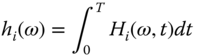
With the defined Hilbert spectrum, the Hilbert marginal spectrum (HMS) of h(ω), can be defined as follows:

where T is the total data length.
The Hilbert spectrum offers a measure of amplitude contribution from each frequency and time value, while the marginal spectrum offers a measure of the total amplitude (or energy) contribution from each frequency value. The marginal spectrum represents the cumulative amplitude over the entire data span in a probabilistic sense. As pointed out in [11], the frequency in the marginal spectrum h(ω) has a totally different meaning from the Fourier spectral analysis. In the Fourier representation, the existence of energy at a frequency ω means there is a component of a sine or a cosine wave persisting through the time span of the data. Here, the existence of energy at the frequency ω only means that in the whole time span of the data, there is a higher likelihood for such a wave to appear locally. In fact, the Hilbert spectrum is a weighted non-normalized joint amplitude-frequency-time distribution. The weight assigned to each time-frequency cell is the local amplitude. Consequently, the frequency in the marginal spectrum indicates only the likelihood that an oscillation with such frequency exists. The exact occurrence time of that oscillation is given in the full Hilbert spectrum.
Therefore, the local marginal spectrum of each IMF component can be given by:
The local marginal hi(ω) spectrum offers a measure of the total amplitude contribution from the frequency ω that we are particularly interested in.
4.2.4 HHT Issues
Although the HHT may become a promising method to extract the properties of nonlinear and nonstationary signals, like other signal analyses, the HHT also suffers from a number of shortcomings. In this section, the limitations of the standard EMD are highlighted.
In order to show the HHT characteristics, an example is given. Consider a simple sine signal as given in (4.12) as shown in Figure 4.2,

Figure 4.2 Test sine signal.
Figure 4.3 and Figure 4.4 show the EMD result and time domain spectrum of the sine signal using the HHT method. Three IMF components and the residue signal are obtained as shown in Figure 4.3. As can be seen from the signal function, it should only get one IMF component. The occurrence of other two IMFs in Figure 4.3 is due to the problems caused by the EMD analysis process.
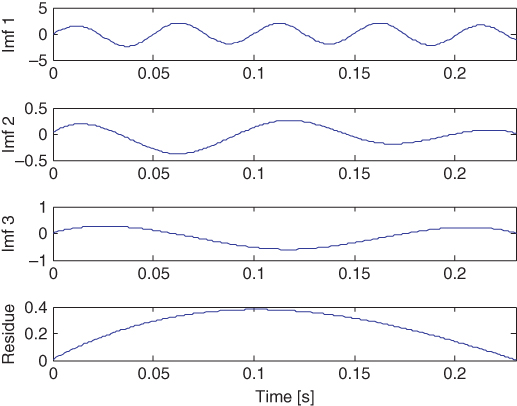
Figure 4.3 EMD analysis result.

Figure 4.4 Time domain spectrum of HHT (Instantaneous frequency).
Figure 4.4 shows the change of three instantaneous frequency components over time. The first frequency component is around 20 Hz, which is similar to the frequency of the test sine signal. However, distortions appear at both endpoints; this phenomenon is called the boundary end effect. The reason for the appearance of the other two instantaneous frequency components, which are called pseudo-IMF components, is discussed in the next subsection.
Before proceeding further, an explanation for a frequency octave is provided. An octave is the frequency range between one frequency and its double or half-frequency. For instance, two frequencies are said to share an octave if their ratio lies between 0.5 and 2. Hence, 0.9 and 1.1 Hz share an octave, while 0.35 and 0.8 Hz lie in different octaves.
Figure 4.5 shows the signal of Eq. (4.13) and its EMD results. It can be seen that the standard application of EMD yields two mono-component IMFs corresponding to the two frequency components (0.4 and 0.175 Hz) in the given signal. Both of them clearly lie in different octaves. However, for the signal of Eq. (4.14), the standard application of EMD fails to yield the two components. The first IMF comes out to be identical to the original signal as shown in Figure 4.6, because the two frequencies (0.5 and 0.375 Hz) lie within the same octave. Thus, the implication is that if a signal contains two modes whose frequencies lie within an octave, standard application of EMD is unable to separate the modes.

Figure 4.5 The signal in Eq. (4.13) (on top) and the first two IMFs (IMF 2 is plotted as dashed line).

Figure 4.6 The signal of Eq. (4.14) (on top) and the first two IMFs (IMF 2 is plotted as dashed line).
From the above signal test, it can be seen that the available HHT algorithms typically include three key issues: (i) boundary end effect; (ii) mode mixing and pseudo-IMF component caused by EMD decomposition, especially for low frequency signals; and (iii) the possibility of parameter identification in power system oscillation analysis. These issues are briefly explained below.
4.2.4.1 The Boundary End Effect
The boundary end effect generated in the EMD process is one of the important factors that affect the quality of EMD. In general, a distortion known as the “Gibbs” phenomenon often appears at signal boundaries when processing signals concentrated in a limited period of time, which is known as the boundary end effect. The Gibbs phenomenon exists for many integral representations [12, 13] as well as for many series representations. The presence of this phenomenon is undesirable, since it is related to the behavior of the series approximating a discontinuous function f at a jump location t, implying a non-uniform approximation at t; so it is important to examine the ways to reduce or even avoid it. In [14] and [15], the Gibbs phenomenon has been shown to exist for Fourier interpolation. Since most multi-resolution analyses induce sampling expansions [16], the Gibbs phenomenon for wavelet sampling expansions has been examined in [17, 18].
In the EMD algorithm, every time “sieve” of a new IMF component has a certain relationship with the old IMF component. Therefore, the distortion at the endpoint will spread to the interior. As a result, the new IMF components obviously have distortion, especially for IMF lower frequency components. This will lead to seriously incorrect EMD decomposition results, and it can also bring endpoint distortion in the Hilbert transform process, which will affect the accuracy of the Hilbert spectrum analysis (HSA). Therefore, solving the boundary end effect issue for the HHT is highly important from both theoretical and practical points of view.
4.2.4.2 Mode Mixing and Pseudo-IMF Component
Mode mixing is defined as a single IMF either consisting of signals of widely disparate scales, or a signal of a similar scale residing in different IMF components [9]. The HHT method defines a unique phase for a real-valued signal at any time instant; it would be easy to compute its rate of change of phase and thereby its frequency. It is possible to define only one instantaneous frequency for a signal at any time instant. This poses a problem for multicomponent signals that have more than one frequency component existing at a given time. The instantaneous frequency obtained for such a signal would be meaningless unless the individual components are isolated before applying the Hilbert transformation. So, if the given signal is an intermittent signal, the mode mixing phenomenon will happen. Many researchers have worked to overcome this problem. One approach proposed is the Ensemble EMD (EEMD), which defines the true IMF components as the mean of an ensemble of trials, each consisting of the signal plus white noise of finite amplitude [19]. Masking signal-based EMD is also an effective method to enhance the discriminating capability of EMD [20, 22]. Besides mode mixing, there are some reasons for generating pseudo-IMF components, such as the boundary end effect, termination criterion for IMF components, and unreasonable sampling frequency selection. After solving the boundary end effect problem, the pseudo-IMF component can be eliminated to some extent.
4.2.4.3 Parameter Identification
It is well known that the EMD method is based on the local characteristic timescale signal. Any signal can be decomposed into the sum of IMF components adaptively in order to make instantaneous frequency have a real physical meaning. Afterward, each IMF component of the instantaneous amplitude and instantaneous frequency can be calculated by the Hilbert transform. In this chapter, the least squares method is employed to combine the HSA and to execute a power system low frequency oscillation parameter identification algorithm. Usually, 10–90% of the IMF component source is used for the identification algorithm. Concerning the poor quality of the IMF components, identification data is used to compress 20–80% of the source IMF components in order to avoid boundary end effects and unstable influence on the two ends caused by the Hilbert transform.
4.3 The Enhanced HHT Method
The HHT algorithm is divided into the EMD process and the HSA process. Removal of direct current (DC) and a band-pass filtering step are needed before applying the HHT algorithm. Since the low frequency oscillations (LFO) or generator rotor angle oscillations have a frequency between 0.1–2.0 Hz [23], the band frequency range is from 0.1 Hz to 2 Hz. The examined signals in the present chapter are: (i) stationary, nonstationary, and possibly nonlinear; (ii) low frequency in the range of 0.1–2 Hz; and (iii) individual component frequencies lying in different octaves.
The proposed improved HHT algorithm is summarized in Figure 4.7. Oscillation signal analysis in power systems is normally decomposed into low frequency oscillation analysis and sub-synchronous oscillation analysis. The IMF components decomposed by the EMD process include the spline interpolation algorithm (cubic spline interpolation function), the endpoint extension algorithm (alternatively direct continuation and mirror extension algorithm), and monotonic constraints (e.g., stop EMD screening process if extreme point is less than 3 and considered residual function is monotonous).

Figure 4.7 Oscillation mode extraction algorithm.
4.3.1 Data Pre-treatment Processing
The signal pre-treatment process includes DC removal and band-pass filtering. First, the DC part of the signal needs to be removed; second, in order to improve the efficiency of analysis, a band-pass filtering algorithm decomposes the useful frequency parts of the oscillating signal processing. Here, “useful” means that the frequency band is 0.1–2 Hz. The DC removal process and band-pass filtering is examined below.
4.3.1.1 DC Removal Processing
The simplest way to removing the DC is to extract the ![]() from the original signal
from the original signal ![]() ; where
; where ![]() is average of xi (t), and
is average of xi (t), and

Hence, the processed signal xi (t) can be written as
4.3.1.2 Digital Band-Pass Filter Algorithm
Here, a Butterworth filter is used as a digital band-pass filter. Compared to the finite impulse response (FIR) filter, the infinite impulse response (IIR) filter offers the advantages of higher efficiency of amplitude-frequency characteristics, desirable accuracy, and low computational effort. Because of phase nonlinearity, it can be also used to analyse power system oscillation effectively.
The Butterworth filter is a type of signal processing filter that is designed to have as flat a frequency response as possible in the pass band. It is also referred to as a maximally flat magnitude filter. It has a magnitude response that is maximally flat in the pass band and monotonic overall. This smoothness comes at the price of decreased roll off steepness. Elliptic and Chebyshev filters generally provide steeper roll off for a given filter order.
The Butterworth filter algorithm can be summarized in five steps:
- a. Find the low pass analog prototype poles, zeros, and gains using the Butterworth filter prototype function.
- b. Convert the poles, zeros, and gain into the state-space form.
- c. Use a state-space transformation to convert the low pass filter into a band-pass, high-pass, or band-stop filter with the given frequency constraints, if required.
- d. Use bilinear transformation method (for digital filter design) to convert the analog filter into a digital filter through a bilinear transformation with frequency pre-warping. Careful frequency adjustment enables the analog and the digital filters to have the same frequency response magnitude at ωn or at ω1 and ω2.
- e. Convert the state-space filter block to its transfer function or zero-pole-gain form, as required.
For the sake of illustration, the following constructed linear/stationary oscillation signal is given as an example:

It contains five frequency components, 0.1 Hz, 0.4 Hz, 2 Hz, 5 Hz, and 15 Hz. After applying the DC preprocessing, the designed 4-order Butterworth band-pass filter (0.1–2 Hz) is used and the result is shown in Figure 4.8. The test data and filtered data are shown in the top and bottom of Figure 4.8, respectively. The FFT method is used to verify the performance of the filter as shown in Figures 4.9 and 4.10. It can be seen that the high frequency (5 Hz and 15 Hz) signals are effectively removed.

Figure 4.8 Pre-treatment process results: test (top) and filtered (bottom) data.

Figure 4.9 FFT spectrum of Butterworth filtered data.

Figure 4.10 FFT spectrum of Butterworth filtered data (zoomed view).
The reliability of the pre-treatment process to cope with nonlinearity/non-stationarity is also tested using the clipped signal. Here, the signal is distorted as given in Eq. (4.18) by clipping its components in some ranges:
The performance of the designed 4-order Butterworth band-pass filter (0.1–2 Hz) can be observed in Figure 4.11. The FFT spectrum is shown in Figure 4.12 in order to verify the performance of the designed filter. The 4 Hz component of the signal has been effectively removed.

Figure 4.11 Pre-treatment process of nonlinear/nonstationary signal results.

Figure 4.12 FFT spectrum of band-pass Butterworth filtered data.
4.3.2 Inhibiting the Boundary End Effect
The boundary end effect of the HHT algorithm is produced for two reasons: one is that, in the EMD process, a cubic spline interpolation exists to strike a mean envelope, in which there is an error at the mean envelope endpoint. The other reason is due to performing the Hilbert transform from the non-integer periodic sampling signal in the HAS, which generates distortion at the endpoint.
4.3.2.1 The Boundary End Effect Caused by the EMD Algorithm
Before introducing the iterated shift process, it is necessary to give a definition of the intrinsic mode function, which must satisfy two conditions. In other words, an IMF is a function that must satisfy two conditions according to the developed algorithm:
- i. The difference between the number of local extremes and the number of zero-crossings must be zero or one.
- ii. The running mean value of the defined envelopes by the local maxima and the local minima is zero.
Condition (i) is used to ensure that the signal has narrow band character, and condition (ii) is applied to assure that the instantaneous frequency does not include the unwanted fluctuations induced by an asymmetric wave.
Furthermore, in the case of using the cubic spline interpolation, the spline should conform to the following stipulations [24]:
- i. The piecewise function S(x) is a third degree polynomial.
- ii. The piecewise function S(x) interpolates all data points
 for
for  .
. - iii. S(x), S′(x), S″(x) are continuous on the interval [x1, xn].
For such a signal, the interior extremes are easily identified. However, at both ends of the data, first or second order derivatives are required for the spline fitting. However, as the data curve does not provide any information on the envelope at the ends, the derivatives cannot be given unless the data is extended beyond the two ends.
To solve this problem, Huang used characteristic waves to get the maximum and minimum extremes [11]. The original signal only has the extreme in the data series, so the external extending points are not reliable. Different characteristic waves cause different results, and it is difficult to choose the proper waves for every iteration.
4.3.2.2 Inhibiting the Boundary End Effects Caused by the EMD
Usually, the extreme points or data sequence at both ends are increased/extended to inhibit the boundary end effect. However, this approach does not provide accurate extrapolating data sequences because of randomness of the real signals. So, it is required to adopt some extension rules to obtain a more accurate mean envelope.
The mirror extension method can be applied in order to solve the boundary end effect problems in the EMD. For the present study, consider the following mathematical expression as the analyzed signal:
The mirror extension method places two mirrors at the left and right end points which give symmetry about the extreme points. Extending the original signal by the mirrors provides a periodic signal sequence. The main steps of the mentioned method are taking the maximum and minimum values of the extended signal, seeking upper and lower envelopes via the cubic spline interpolation function, and finally seeking the average of the envelope.
The result of the EMD process applying a mirror extension method is shown in Figure 4.13. Comparing this with Figure 4.4, Figure 4.14 shows the boundary end effect problem of the EMD algorithm is properly inhibited by the mirror extension method. At the same time, pseudo-IMF components are also eliminated in this example.

Figure 4.13 The mirror extension method.

Figure 4.14 Inhibiting the boundary end effect problem of the EMD algorithm by the mirror extension method.
4.3.2.3 The Boundary End Effect Caused by the Hilbert Transform
The error of instantaneous frequency and amplitude calculated in the Hilbert transform causes some impacts on the final results of the analysis, including the parameter identification quality. In what follows, the Hilbert transform of a sine signal given by (4.12) and its frequency spectrum is calculated to observe the boundary end effect resulting from the Hilbert transform.

Figure 4.15 Non-integral periodic sine signal and its Hilbert transform (T=0.23).

Figure 4.16 Instantaneous frequency of non-integral periodic sine signal.
Applying the Hilbert transform to the signal, the signal waveform and its Hilbert transformed wave are obtained as shown in Figure 4.15. It is known that there is π/2 phase difference between a sinusoidal signal and the Hilbert transform result. It is clear that the error generated by the Hilbert transform is reflected in the instantaneous frequency spectrum, which is shown in Figure 4.16. As can be seen, a serious distortion occurs at the endpoints.
To inhibit the endpoint distortions, the reasons of this distortion must be understood first. As shown in Figure 4.17, the Hilbert transformation process provides a bilateral spectrum of the real signal by applying Fourier transform. Then, filtering is used to remove one side of the spectrum, and the amplitude is doubled. Finally, applying the inverse Fourier transform to the doubled unilateral spectrum produces the final result.

Figure 4.17 HT computing process.
The core element throughout this process is the Fourier transform. The Fourier transform is used for periodic signals. Therefore, for a signal with non-periodic data series, the result will be mixed with error terms.

Figure 4.18 Integral periodic sampling sine signal and its Hilbert transform.
Figure 4.18 shows the results of Hilbert transform application to the integral periodic sampling of the sine signal (4.12). Comparing this with the non-integral periodic sampling data sequence in Figure 4.15, it can be seen that through the Hilbert transformation, a non-positive periodic sampling at the endpoint is distorted rather than the integral periodic sampling sequence.
Although it is known that the endpoint distortion can be inhibited by sampling integral periodic for the signal, it is very difficult to integrate periodic sampling of data in a real complex project. Therefore, it is necessary to use other methods to inhibit the boundary end effect produced by the Hilbert transformation.
4.3.2.4 Inhibiting the Boundary End Effect Caused by the HT
The boundary end effect produced by the Hilbert transform mainly appears at the ends of data series. The Hilbert transform results can be approximately obtained by shifting ± π/2 phase to the original signal. So the ends of the original data can be extended according to certain rules, and then the Hilbert transform can be applied to the new extended data. Finally, after removing the Hilbert transform results at the extension data parts, the rest of the data is the Hilbert transform results of the original data. The most important part of this approach is the method selection for data extension. In this research, the autoregressive moving average (ARMA) model method is selected to establish extension data.
For some observed time series, a high-order autoregressive (AR) or moving average (MA) model is needed to model the underlying process. In this case, sometimes a combined ARMA model can be a more parsimonious choice.
An ARMA model expresses the conditional mean of yt as a function of both past observations, yt − 1,…,yt − p, and past innovations, ϵt − 1,…, ϵt − q. The number of past observations (yt) depends on p, which is the AR degree. The number of past innovations (yt) depends on q, which is the MA degree. In general, these models are denoted by ARMA (p, q).
The form of the ARMA (p, q) model is [25]:
where ϵt is a white noise signal (uncorrelated innovation with mean zero).
Define the AR(p) and MA(q) as lag operator polynomials ![]() and
and ![]() , respectively. The ARMA (p, q) model can be written as
, respectively. The ARMA (p, q) model can be written as
where ![]() . The signs of the coefficients in the AR lag operator polynomial φ(L) are opposite to the right hand side of Eq. (4.20).
. The signs of the coefficients in the AR lag operator polynomial φ(L) are opposite to the right hand side of Eq. (4.20).
The basic consideration to extend the ends of the original data according to the ARMA method is given in an algorithm that is summarized in Figure 4.19. Based on this algorithm, firstly the ARMA model to extend the original data is established. Then the Hilbert transform is performed, and finally the Hilbert transform (HT) results of the original signal are intercepted.

Figure 4.19 Inhibiting the boundary end effect algorithm.
Comparing this with Figure 4.16, the distortions at both ends of the instantaneous frequency spectrum of non-periodic sampling signals are effectively inhibited after applying this algorithm, as shown in Figure 4.20.

Figure 4.20 Processed instantaneous frequency spectrum.
4.3.3 Parameter Identification
In power systems, the oscillation mode component can be written as:
or
where A is initial amplitude, ψ is initial phase, λ is damping coefficient, ω is oscillation angular frequency, f is oscillation frequency, ω0 is un-damped angular frequency, ωd is damped angular frequency, and ξ is damping ratio.
Comparing Eqs. (4.22) and (4.23) gives:

For identification of the frequency oscillation signal, it is necessary to accurately extract the amplitude of the oscillation component and damping coefficient, and then calculate the damping ratio, which depends on the oscillation frequency and damping factor.
The frequency oscillation signal exists in the decomposed IMF components as an oscillation mode component. Therefore, parameter identification is needed. In order to obtain more accurate identification results, two issues should be considered. The least squares method is used to improve the accuracy of the damping coefficient and oscillation amplitude. It is also necessary to make some changes in the analytical signal form as shown in Eq. (4.25). Damping coefficient (λ) identification uses least squares through the logarithmic curve of instantaneous amplitude function of a single IMF component.

On the other hand, reducing the IMF component data is also noteworthy. Since the data for parameter identification is obtained from the IMF component, the boundary end effect caused by the EMD is suppressed, but is not fully eliminated. At the same time, the endpoint distortion coming from the Hilbert transform is also not completely eliminated. Therefore, IMF can improve identification accuracy by removing small amounts of data at the both ends. In this work, 10–90% of the IMF component source is used for the identification algorithm.
4.4 Enhanced HHT Method Evaluation
4.4.1 Case I
The effectiveness of the proposed algorithm is used by application to the given oscillation signal in (4.17). This signal contains power system frequency components including inter-area oscillation (0.1–1 Hz), local oscillation (1–2 Hz) and noise oscillation (over 2 Hz).
This section also addresses the effect of the sampling time applied by the enhanced EMD algorithm. The results are shown in Figs. 4.21 and 4.22, with sampling time of 0.01 s and 0.033 s, respectively. Both figures include three oscillation modes and one residue. The frequencies of IMF components from high to low are 2 Hz, 0.4 Hz, and around 0.1 Hz. Comparing two results with different sampling times, it is easily to see that serious distortion occurred in the low frequency component with sampling time of 0.033 s (Figure 4.22), especially at the lowest frequency of 0.1 Hz. The reason for this distortion is the Gibbs phenomenon in the Butterworth filter processing, which is introduced in Section 4.3.1.
It is well known that low frequency oscillation in power systems is much more threatening than high frequency oscillation. In order to inhibit the distortion caused by Butterworth filter processing, the signal is analyzed without pre-treatment. Figure 4.23 for sampling time of 0.01 s and Figure 4.24 with sampling time of 0.033 s shows the EMD result without pre-treatment.
Figure 4.23 includes five oscillation modes and one residue at a sampling time of 0.01 s. The frequencies of IMF components from high to low are 15 Hz, 5 Hz, 2 Hz, 0.4 Hz, and around 0.1 Hz. The residue DC component is 15. Figure 4.24 includes four oscillation modes and one residue at a sampling time of 0.033 s. The frequencies of IMF components are 5 Hz, 2 Hz, 0.4 Hz, and around 0.1 Hz. The residue DC component is 15. It can be found that regardless of the sampling time, there are no serious distortions in the low frequency component. However, the high frequency component cannot be observed in the low sampling time cases.
From Figs. 4.21 and 4.22, it can be seen that the pre-treatment process can help to cut down noise performance and high frequency components. In the low sampling time cases, the pre-treatment process has worked, but without a high accuracy in the low frequency components (see Figs. 4.22 and 4.24).

Figure 4.21 Pre-treatment EMD results (sampling time 0.01s).

Figure 4.22 Pre-treatment EMD results (sampling time 0.033s).
In conclusion, these two comparisons indicate that by applying pre-treatment, the effects on the results are removed in high sampling time cases, while in the low sampling time situation, high frequency elements cannot be observed but low frequency distortion has happened. To observe low frequency components correctly at high sampling times, a pre-treatment process is needed. On the other hand, to observe low frequency elements clearly in low sampling time cases, the pre-treatment process should not be applied.

Figure 4.23 EMD results (sampling time 0.01s).

Figure 4.24 EMD results (sampling time 0.033s).
4.4.2 Case II
In this case, a constructed bimodal oscillation signal including damping coefficients is defined as follows:
This oscillation signal, shown in Figure 4.25, contains three decay elements with damping coefficients of -0.15, -0.2, and -0.1 and frequencies of 2 Hz, 1 Hz, and 0.4 Hz; and a DC component of 15. Here, we can get the IMFs by applying the improved EMD algorithm as shown in Figure 4.26. Table 4.1 shows the identified parameters for each IMF component. It can be seen that the improved HHT method can estimate the frequencies, damping coefficient, and damping ratio of the three modes effectively. Moreover, the estimation results are not affected by the sampling time. From the results, it can be concluded that the improved HHT algorithm effectively decomposes the low frequency oscillation signal mode. The correct oscillation parameters can be obtained from the decomposed modal signal without considering the sampling time. This is an effective method for low frequency oscillation signal analysis as long as it can be correctly extracted.
Table 4.1 Parameter identification results
| Mode | Frequency | Damping Coefficient | Damping Ratio | |||
| Sampling Time(s) | 0.01 | 0.033 | 0.01 | 0.033 | 0.01 | 0.033 |
| 1 | 2.0800 | 2.0766 | −0.1490 | −0.1516 | 0.0118 | 0.0120 |
| 2 | 0.9936 | 0.9951 | −0.1948 | −0.1978 | 0.0310 | 0.0315 |
| 3 | 0.3917 | 0.3903 | −0.1032 | −0.1000 | 0.0419 | 0.0407 |

Figure 4.25 Bimodal test oscillation signal.

Figure 4.26 EMD results of bimodal test signal given in (4.26).
4.4.3 Case III
The reliability of the proposed algorithm to deal with nonlinear/nonstationary signals is investigated by application to the oscillation signal given in Eq. (4.18), distorted by clipping its components in some ranges. This signal contains power system frequency components including inter-area oscillation (0.4 Hz), local oscillation (1.1 Hz) and noise oscillation (4 Hz). The decomposition performance with enhanced EMD algorithm can be observed in Figures 4.27 and 4.30 with a sampling time of 0.033 s. It can be seen that IMF 1 and IMF 2 in Figure 4.27 and IMF 1, IMF 2, and IMF 3 in Figure 4.28 preserve the frequency of each corresponding component, while at the same time trying to capture the shape of the distorted signals, respectively. Both decompositions yield another two insignificant IMFs plus a residue. In order to show the difference analysis performance, Figure 4.29 shows the first two IMFs of the distorted signal obtained with pre-treatment EMD compared with original test signal, Figure 4.30 demonstrates that the IMF 2 and IMF 3 of the distorted signal are obtained without pre-treatment of the EMD and the original test signal.

Figure 4.27 Pre-treatment EMD results.

Figure 4.28 EMD results.

Figure 4.29 The first two IMFs of the distorted signal obtained with pre-treatment EMD.
From the quantities shown in Tables 4.2 and 4.3, it can be seen that the HHT without pre-treatment is more reliable than the pre-treatment one in dealing with nonlinearities (here, the clipped signals). While, the higher order IMFs and the residue from HHT are insignificant in terms of magnitudes with respect to IMF 1 and IMF 2 through the pre-treatment process and to IMF 1, IMF 2, and IMF 3 with EMD-based filtering, which represent the components of the signal. The extra components yielded by EMD-based filtering have lower values than the applied pre-treatment. Moreover, the damping coefficient and ratio computation show that the EMD-based filtering is more accurate than the pre-treatment process.
Table 4.2 Parameter identification results with pre-treatment
| Mode | Frequency | Damping Coefficient | Damping Ratio |
| 1 | 1.1260 | −0.0109 | 0.0016 |
| 2 | 0.3327 | −0.0256 | 0.00129 |
| 3 | 0.1638 | −0.0078 | −0.0497 |
| 4 | 0.0980 | 0.0528 | −0.0900 |
Table 4.3 Parameter identification results with EMD-based filtering
| Mode | Frequency | Damping Coefficient | Damping Ratio |
| 1 | 3.917 | 0.0038 | −1.6185e-4 |
| 2 | 1.0916 | −0.0017 | 2.5716e-4 |
| 3 | 0.2976 | −0.0013 | 7.008 e-4 |
| 4 | 0.1311 | −0.0206 | 0.025 |
| 5 | 0.0645 | 0.0313 | −0.0672 |

Figure 4.30 IMF 2 and IMF 3 of the distorted signal obtained without pre-treatment EMD.
4.5 Application to Real Wide Area Measurements
Generally, according to power system network structure and generator distribution, only one or two oscillation modes join together to dominate overall system dynamics. Furthermore, it is more common that for a studied system there is only one dominant oscillation mode which significantly influences overall system dynamics. The dominant oscillation mode can be separated from original measurements, and the problem is reduced to a parameter estimation problem of a single oscillation mode [1].
The Japan power network is used as a case study. Due to the longitudinal structure of this network, there are some significant low frequency oscillation modes across the whole system. Recently, a joint research project has been presented between some universities in Japan to develop an online wide area measurement of power system dynamics by using synchronized phasor measurement technique [3].
To establish a real WAMS, 13 PMUs are installed in universities/institutes in different geographical locations of Japan [3]. The PMUs are synchronized by the global positioning system (GPS) signal. This project was started to develop a WAMS covering the whole power system in Japan as a collaborative research initiative called Campus WAMS as shown in Figure 4.31. The PMUs measured voltage phasors in the monitoring location (laboratory) of the assigned university campuses over 24-hour schedules.

Figure 4.31 PMU locations for the Campus WAMS project (Japan).
The Campus WAMS was developed to cover the typical power supply areas of the entire Japanese national-wide power grid. At least one PMU is installed in the supply network of each power company. Currently, the Campus WAMS project encompasses 13 PMUs (10 PMUs are installed in the supply area of the Western Japan 60-Hz system and 3 PMUs are located in the supply area of the Eastern Japan 50-Hz system). The locations of these PMUs are marked with filled circles associated with the respective city name in Figure 4.31. All PMUs are of the same model (NCT2000 Type-A manufactured by Toshiba Corp.), which is shown in Figure 4.32 [26].

Figure 4.32 Phasor measurement unit (Toshiba NCT2000).
The main objective of this section is to present a monitoring and estimation scheme for power system inter-area oscillation based on wide area phasor measurements from the Campus WAMS. This scheme only focuses on the estimation of single dominant inter-area oscillation mode and includes the following steps: (i) estimating the center frequency of the single mode of interest, (ii) extracting the oscillation data from the original phasor measurements, (iii) analyzing the oscillation shape, (iv) identifying the oscillation model, and (v) estimating the oscillation parameters. Without considering any additional disturbance intentionally imposed on the system, a simplified second order oscillation model can be derived and identified based on the extracted oscillation data corresponding to the targeted single oscillation mode. The EMD-based filter technique is employed to separate the targeted single oscillation mode from other existing modes. The Hilbert marginal spectrum (HMS) analysis technique introduced in Section 4.2.3 is adopted to determine this center frequency from the original phasor measurements of power system output variables. Here, the center frequency means the real oscillation frequency of the targeted inter-area mode.
Figure 4.33 shows the waveforms of phase difference between Miyazaki University and Tokushima University stations. The twelve IMFs and one residue of the phase difference obtained using the EMD are listed in Figure 4.34. The frequencies of the IMFs are ordered from high to low. The HMS technique is adopted to determine the real oscillation frequency of the targeted inter-area mode, which is demonstrated in Figure 4.35. The oscillation mode can be extracted in the frequency range of 0.3–0.5 Hz. Then, the oscillation shape of a short period of data from the extracted oscillation mode (FFT filtered) [3, 26] and obtained IMF 5 (EMD filtered) are compared with the original phasor difference (Figure 4.36). It can be seen that the EMD filter can estimate the local characteristic more accurate than the FFT filter. The maximum amplitude value is extracted from the amplitude of the oscillation mode frequency range (Figure 4.37).

Figure 4.33 Waveforms of phase difference between Miyazaki University and Nagoya Institute of Technology University stations.

Figure 4.34 EMD results.

Figure 4.35 Hilbert marginal spectrum.

Figure 4.36 Short time phasor difference data from the extracted oscillation mode (FFT filtered) and obtained IMF 5 (EMD filtered).

Figure 4.37 Amplitude of the extracted oscillation mode.
Figure 4.38 shows the time domain data from the extracted oscillation mode at the maximum point, which is used to estimate the power system oscillation parameters. In this case, the total computation time is less than two seconds. The resulting estimated parameter values for power system frequency oscillation are angular frequency (3.4344 rad/s), damping coefficient (-0.06891), and damping ratio (0.0820). Finally, the FFT filter-based process calculates the same oscillation mode characteristics, resulting in an angular frequency of 2.9762 rad/s and damping ratio of 0.0543.

Figure 4.38 Short time data from the extracted oscillation mode and the obtained IMF.
4.6 Summary
In recent years, detecting and analyzing the low frequency oscillation phenomenon in power systems has become an attractive research topic. As a result, many experts and scholars around the world have done valuable research work in the field of power system time-frequency analysis and have developed numerous processing methods for the oscillation signals.
In the present chapter, an integrated scheme based on an enhanced HHT algorithm is introduced for monitoring and detecting low frequency oscillations. Several key signal processing techniques are implemented to improve the HHT method. The relevant central frequency of the relevant mode is determined automatically and accurately, and this is then used to determine the oscillation mode parameters. The extracted frequency mode, damping, and oscillation shape can be properly detected by the proposed oscillation monitoring scheme.
References
- 1 Bevrani H., Watanabe M., and Mitani Y., Power System Monitoring and Control, Wiley-IEEE Press, New York, USA, 2014
- 2 Tsukui R., Beaumont P., Tanaka T., and Sekiguchi K., “Intranet-based protection and control”, IEEE Com-put Applications in Power, vol. 14, no. 2, pp.14–17, 2001
- 3 Hashiguchi T., Yoshimoto M., Mitani Y., Saeki O., and Tsuji K., “Oscillation mode analysis in power systems based on data acquired by distributed phasor measurement units”, Proceedings of the 2003 IEEE International Symposium On Circuits And systems, 2003
- 4 Walter, G.G., Wavelets and Other Orthogonal Systems With Applications, CRC Press, 1994
- 5 IEEE Publications, “Identification of Electromechanical Modes in Power Systems”, IEEE Power & Energy Society, Special publication TP462, June 2012.
- 6 Messina, A.R., Vittal V., Ruiz-Vega D., and Enríquez-Harper G., “Interpretation and visualization of wide-area PMU measurements using Hilbert analysis”, IEEE Trans. on Power Systems, vol. 21, no. 4, November 2006, pp. 1763–1771.
- 7 Liu Q., Watanabe M., and Mitani Y., “Global oscillation mode analysis using phasor measurement units-based real data”, International Journal of Electrical Power & Energy Systems, vol. 67: pp. 393–400, 2015
- 8 Browne T.J., Vittal V., Heydt G.T., and Messina A.R., “A comparative asse ssment of two techniques for modal identification from power system measurements”, IEEE Trans. on Power Systems, vol. 23, no. 3, 2008, pp. 1408–1415.
- 9 Huang N.E., and Shen, S.S.P. (eds), “The Hilbert–Huang Transform and Its Applications”, 2nd Edition, World Scientific Publishing Company pp.1–15, 2005
- 10 Heisenberg W., “Über quantentheoretishe Umdeutung kinematisher und mechanischer Beziehungen”, Zeitschrift für Physik, 33, 879–893, 1925 (received July 29, 1925). English translation in: B. L. van der Waerden, Sources of Quantum Mechanics, NorthHolland publishing company, Amsterdam, Holland, 1967.
- 11 Huang N.E., Shen Z., Long S.R., et al, “The empirical mode decomposition and the Hilbert spectrum for nonlinear and non-stationary time series analysis”, Proceedings of the Royal Society London, Series A, 454(1998) 903–995
- 12 Jerri A., “The Gibbs Phenomenon in Fourier Analysis”, Splines and Wavelet Approximations, Kluwer Academic Publishers, 1997
- 13 Karanikas C., “Gibbs phenomenon in wavelet analysis”, Result. Math., vol. 34, pp. 330–341, 1998
- 14 Helmberg G., “The Gibbs phenomenon for Fourier interpolation”, J. Approx. Theory, vol. 78, pp. 41–63, 1994
- 15 Helmberg G. and Wagner P., “Manipulating Gibbs' Phenomenon for Fourier interpolation”, J. Approx. Theory, vol. 89, pp. 308–320, 1997
- 16 Atreas N.D., and Karanikas C., “Gibbs Phenomenon on sampling series based on Shannon's and Meyer's wavelet Analysis”, Fourier Analysis and Applications, vol. 5, no. 6, pp. 575–588, 1999
- 17 Shim H.T., Volkmer, “On the Gibbs Phenomenon on wavelet expansions”, J. Approx. Theory., vol. 84, no. 1, pp. 74–95, 1996
- 18 Walter, G.G., and Shim, H.T., “Gibbs Phenomenon for sampling series and what to do about it”, Fourier Analysis and Applications, vol. 4, no. 3, pp. 357–375, 1998
- 19 Wu Z., and Huang, N.E., “Ensemble Empirical Mode Decomposition: a noise assisted data analysis method”, p. 1, 2005
- 20 Deering R., “Fine -scale analysis of speech using empirical mode decomposition: Insight and applications,” PhD Thesis, Department of Mathematics, Duke University, USA, 2006.
- 21 Deering R., and Kaiser, J.F., “The use of a masking signal to improve empirical mode decomposition,” 2005 IEEE International Conference on Acoustics, Speech and Signal Processing, March 2005.
- 22 Laila D.S., Messina A.R., and Pal B.C., “A refined Hilbert–Huang transform with application to interarea oscillation monitoring” IEEE Trans. on Power Syst. EMS, vol. 24, no. 2, pp. 610–620, May 2009,
- 23 Kundur P., “Power System Stability and Control”, (McGraw-Hill: New York, 1994)
- 24 Hazewinkel M. (ed.), “Spline interpolation”, Encyclopedia of Mathematics, Springer, ISBN 978-1-55608-010-4, 2001
- 25 MathWorks, Matlab, http://www.mathworks.com/products/matlab
- 26 Mitani Y., Saeki O., Hojo M., and Ukai H., “Online monitoring system for Japan Western 60 Hz power system based on multiple synchronized phasor measurements”, Papers of Technical Meeting on Power Engineering and Power System Engineering, IEE Japan, PE-02-60, PSE-02-70, 2002 (in Japanese)