Chapter 4
Reliability
Chicken buses.
For the uninitiated, they're the decommissioned big, yellow school buses, shipped, driven, or towed south from the United States to Guatemala for a new life and revitalization. But to be reborn as a chicken bus, you need four things—chickens, color, bling, and exhaust.
With large segments of the Maya people living in fairly remote, inaccessible regions, public buses are largely favored over personal vehicles in highland pueblos. As an agrarian people, the Maya transport not only their produce but also their livestock to large communal markets twice or thrice weekly. I've encountered live chickens on chicken buses several dozen times—but also goats, sheep, and one “dog” that was so ugly I still believe a family was bussing their chupacabra to market to sell.
The Guatemalan highlands are the most colorful landscape and people I've ever encountered, boasting the largest concentrations of ethnic Maya in the world. The orchidaceous colors woven for centuries into their textiles are vibrantly reincarnated on the buses that crisscross the landscape's mountainous roads. Vibrant paintings of saints, the Virgin Mother, and biblical quotations are common chicken bus adornments, as are tie-dye and Christmas themes.
Every bus is also chromed to the max—its grill, bumper, and wheels, naturally, but also vintage air horns, Mercedes and Rolls Royce emblems, and spurious smoke stacks, ladders, railings, and anything else that can be polished to a mirrored finish. That is to say that despite the cobblestone and dirt roads that chicken buses must daily navigate, their exteriors are impeccably maintained.
As for the exhaust—well, Guatemala boasts neither the emission standards nor maintenance requirements of the United States, so plumes of black smoke trail nearly all the buses, while passengers are left to subtly choke and question the integrity and reliability of the service.
I was en route from Antigua to Panajachel, the largest pueblo bordering the pristine Lake Atilán. We'd endured the groaning engine, straining gears, and tumultuous shifting for nearly two hours—not to mention the stench of livestock—when finally the chicken bus slowed on an uphill climb and drifted off the road to a halt. After 20 minutes of commotion, we were ordered to disembark. No, it wasn't the bandidos (bandits) this time, just another engine gone awry.
Now I never heard the original instructions from the conductor (driver), over the braying sheep and brash cry of infants, but as I strode around the roadside with my 100 companions, it was clear that we were supposed to be searching for something. But what?
A young student, amused with my consternation, finally translated that we'd been ordered to scour the countryside for—now wait for it—pieces of metal and twine.
I watched with a mixture of respect and fear as the conductor tinkered in the engine and “repaired” our chicken bus with roadside twine and other sundry scraps that had been gathered by passengers. An hour later, we were again slowly making our way to the lake, everyone seemingly undaunted by the day's events. They'd undoubtedly seen this scene play out enough times that it neither raised eyebrows nor diminished spirits. We'd reach Pana when we reached Pana.

To many Guatemalans, chicken bus reliability is not a priority in life. They do value bus security (i.e., no bandidos), but if a bus picks them up hours late or breaks down en route, they don't get too ruffled. In fact, they're happy to pitch in and search the brush for metal, twine, and other scraps and to lend a helping hand to unexpected roadside maintenance.
In many end-user development environments, software reliability is not valued as highly as other quality characteristics. Especially in data analytic development environments, emphasis is placed on getting the right data and analytic solution, but not necessarily on producing software that can run reliably without assistance or regular maintenance.
If software encounters unpredictable exceptions or otherwise fails, SAS practitioners often can fix it on the spot without additional assistance. They may have been the original developers of the software but, even if not, as software developers, SAS practitioners are able to get their software back on the road.
Thus, in some ways, end-user software development mimics chicken buses in that the conductor is expected not only to be a formidable driver, but also to maintain the bus. The benefits are great, because a skilled conductor who can moonlight as a mechanic is more likely to discern when a bus is running poorly, struggling, and about to fail. And, with this mechanical knowledge of the bus, he's often able to get the bus—for better or for worse—running again without a tow.
Because data analytic developers understand not only their industry and business through domain expertise, but also software development, they're more likely to detect when software is running poorly or producing invalid output or data products. Following detection of runtime errors, SAS practitioners are able to gather the necessary scraps to get their code functioning again.
A downside of data analytic development, however, is its reliance not on the integrity of software but on the end-user developers themselves who maintain it. Build software for a third-party and separate the developers from the users so the two never shall meet, and users must trust that software will be reliable, consistent, and provide accurate results for its intended lifespan. But imbed users with developers (including end-users who are developers), and software reliability typically plummets because reliability is instead placed in the people, not the software.
This chapter introduces software reliability which requires a shift from trusting in the personnel who maintain software to trusting in the software itself to be robust to failure, to function consistently, and to perform for its intended lifespan without excessive maintenance or modification. A hallmark of reliable SAS software is that it can be executed if necessary by non-developers with minimal Base SAS knowledge.
DEFINING RELIABILITY
Reliability is defined in the International Organization for Standardization (ISO) software product quality model as “the degree to which the software product can maintain a specified level of performance when used under specified conditions.”1 The Institute of Electrical and Electronics Engineers (IEEE) additionally includes the concept of software endurance or longevity, defining reliability as “the ability of a system or component to perform its required functions under stated conditions for a specified period of time.”2 Historical definitions typically incorporated failure into reliability—for example, “the probability that software will not cause the failure of a system for a specified time under specified conditions.”3
A more general definition of reliability is a measure of performance against failure, often defined mathematically as the probability of error-free operation. A reliable product or service can be depended upon to deliver expected functionality and performance in a consistent, repeatable manner and for some expected duration. Because an unreliable product is often considered worthless, reliability is typically considered paramount to other performance requirements. Within the ISO software product quality model, the reliability dimension additionally includes subordinate characteristics of availability (described in this chapter), fault-tolerance (described in chapter 5), and recoverability (described in chapter 6).
The ACL triad that includes availability, consistency, and longevity is introduced, demonstrating qualities that reliable software must espouse. Software failure and the risk thereof are explored through the contributing effects of errors, exceptions, defects, faults, threats, and vulnerabilities. Through reliable software, SAS practitioners demonstrate their technical prowess and earn the trust and respect of stakeholders who learn to trust the software—not only the maintenance skills—of their developers.
PATHS TO FAILURE
If failure distinguishes reliability from unreliability, it's important first to define software failure and distinguish this from other related, often commingled terms, including defect, fault, bug, and error. Software reliability is ultimately judged from the perspective of the customer or sponsor, the source of software requirements. Failures are identified as customers detect software deviations from stated requirements, and as users detect deviations from software marketing, instruction, and other documentation. Failure can also be interpreted and defined differently based on stakeholder perspective, as demonstrated in the “Redefining Failure” section in chapter 5, “Recoverability.”
Because reliability can be thwarted by functional or performance failures and because numerous pathways lead to software failure, some differentiation between these terms is beneficial. The accompanying textbox defines failure-related software development terms. In this text, defect is used to represent incorrect code that causes a failure, in keeping with IEEE definitions. Errors are distinguished from defects, with the former causing the latter, described in the following section.
Errors, Exceptions, and Defects
In most software literature, errors are described as some variation of human-derived mistakes. Errors are not limited to code and in fact often point to derelict, incomplete, or misconstrued software requirements. Errors can also occur when incomplete or otherwise invalid data or inputs are received. The entry of invalid data into software can signal errors in data entry or data cleaning processes but if the software was intended to be reliable, the inability of SAS software to detect and handle invalid data appropriately represents another error—the lack of quality controls.
Errors printed to the SAS log are referenced in this text as runtime errors to distinguish them from the IEEE definition of error, which reflects a human mistake. Runtime errors can occur when SAS practitioners make errors in code (syntax errors) or for various reasons such as out-of-memory conditions. When SAS runs out of memory (and produces a runtime error), the underlying error (human mistake) could represent inefficiently coded SAS syntax, the failure of requirements documentation to state memory usage thresholds, or the failure of a SAS administrator to procure necessary memory. Thus, the source of runtime errors may not be programmatic in nature despite causing programmatic failure.
The SAS Language Reference lists several types of errors that can occur in software, including syntax, semantic, execution-time, data, and macro-related.11 Syntax errors, for example, occur when invalid or imperfectly formed code is executed, a common example being the infamously missing semicolon:
data final
   set original;
run;
For the purpose of this text, syntax and semantic errors are not distinguished because they represent invalid code that should not exist in production software and which likely will have been discovered during software testing. In this example, the error—the missing semicolon—can also be considered the defect, because the code is corrected by adding the semicolon, which prevents further software failure.
Exceptions occur when software encounters an unexpected, invalid, or otherwise problematic environmental state, data, or other element or action. For example, if data standards specify variable value ranges, receiving invalid data beyond those ranges represents an exception. Or if SAS software is designed and developed to run on Windows, an exception occurs when SAS encounters a UNIX environment. Exceptions are described in the section “Exception Handling” in chapter 6, “Robustness,” which demonstrates methods to detect and handle exceptions to facilitate robust, reliable execution.
Some software exceptions are automatically handled by Base SAS native exception handling routines, such as division-by-zero detection, which prints a note to the SAS log that a zero denominator was detected but does not produce a runtime error. In fact, one of the primary goals of exception handling is to detect some abnormal state (like a zero denominator) and prevent a runtime error from occurring. Base SAS has very few native exception-handling capabilities, so in most cases developers will need to build an exception-handling framework that forestalls exceptional events and other vulnerabilities that can cause software failure.
A division-by-zero exception is detected and handled natively by Base SAS, which converts the attempted fraction to a missing value, as demonstrated in the following output:
data temp;
   num=5;
   denom=0;
   div=num/denom; * div set to missing;
run;
NOTE: Division by zero detected at line 1786 column 12.
num=5 denom=0 div=. _ERROR_=1 _N_=1
NOTE: Mathematical operations could not be performed at the following places. The results of the operations have been set to missing values.
Because SAS contains built-in exception handling to detect division by zero, a note rather than error is printed to the log, and both the automatic macro values for &SYSCC and &SYSERR remain 0, representing error-free execution. If this is the intended outcome of division by zero, it's acceptable to allow SAS native exception handling to handle division by zero. Thus, in the previous example, no additional user-defined exception handling is required because the missing value is desirable.
In other cases, however, software requirements might specify that native exception handling is not sufficient. For example, rather than setting a value to missing, perhaps the entire observation should have been deleted. The zero value might indicate that more substantial data errors exist elsewhere, requiring termination of the process or program. In these cases, division by zero could represent not only an exception, but also a failure caused by software errors.
In some cases, division by zero can be caused by faulty or missing exception handling that fails to detect the zero denominator before division. In the following example, exception handling attempts to prevent division by zero but, due to a typographical error, instead eliminates values of one. Thus, while the exception—the division by zero—occurs in line four, line three contains the typographical error and thus the defect that must be corrected:
data final;
   set original;
   if denomˆ=1 then do;   * typographical error and defect occur here;
      div=num/denom;   * exception occurs here;
      end;
   else delete;
run;
Another version of the division-by-zero exception occurs when exception handling to detect a zero denominator was omitted because no quality control check was specified in software requirements. Thus, while the exception occurs in line three of the code, the real error is a failure of creativity in software requirements: SAS practitioners overlooked the possibility that zero values could be encountered. During software design, protocols for exceptional data should be discussed so that software can respond in a predictable manner if they are encountered:
data final;
   set original;
   div=num/denom;   * execution error occurs here;
run;
A final version of the division-by-zero exception occurs when quality control (to prevent zero denominators) was incorporated into requirements but the requirements were not implemented. For example, perhaps the requirements stated that the first DATA step (which creates Original) should delete all observations for which the value of Denom was 0 or missing. However, because this quality control was omitted, an exception occurs in the second module when invalid data are passed that include zero Denom values. This error ultimately represents a failure in communication or interpretation of technical requirements:
* MODULE 1;
data original;
   set temp;   * error (omission of quality control) occurs here;
run;
* MODULE 2;
data final;
   set original;
   div=num/denom;      * exception occurs here;
run;
In this scenario, software requirements prescribe that data quality controls should have been placed in the first module, so the overarching error occurs here, as well as the defect that should be corrected. However, this error goes undetected in the first DATA step because the exception—the division by zero—does not occur until the second module. To remedy the exception, the defect in the first DATA step can be corrected by implementing the required exception handling there, or the requirements can be modified so that the exception handling can be implemented in the second DATA step. Either solution will correct the failure, but this demonstrates that exception- and error-causing code can often be defect-free while pointing to defects and errors in separate code or modules.
While division by zero represents a handled exception, many runtime errors are caused by unhandled exceptions. For example, the DELETE procedure was introduced in SAS 9.4, so use of the procedure in previous SAS versions will cause runtime errors and software failure. For SAS practitioners who implement the DELETE procedure in code, exception handling would be required to make the software portable to previous versions of SAS, possibly by instead deleting data sets with the DATASETS procedure. In this way, while the exception—encountering SAS 9.1—still occurs, it is detected and handled, preventing runtime errors and software failure. This practice is discussed further in the “SAS Version Portability” section in chapter 10, “Portability.”
Failure
Failure occurs when software does not function as needed, as intended, or as specified in technical requirements. A functional failure occurs when software does not provide the specified service, result, or product. In data analytic development, SAS software is often developed to produce an analytic product that may incorporate separate data ingestion, cleaning, transformation, and analysis steps. If the ultimate analysis is incorrect due to errors in any of these steps, this represents a functional failure because the intent of the software—the analytic product—is invalid.
In the scenario in the “Errors, Exceptions, and Defects” section, the failure to delete observations that contained a division by zero is a functional failure because the software creates an invalid data product. On the other hand, when the analysis is correct but is produced more slowly than specified by technical requirements, this instead represents a performance failure. Because this text focuses on the performance side of quality, unless otherwise specified, all scenarios and code examples depict fully functional solutions that deliver full functionality and valid data products; all failures represent performance failures.
In addition to producing incorrect behavior, a software failure by most definitions must also be observable—not necessarily the cause, but at least the effect. That a failure can be observed, however, does not indicate that it has been observed; as a result, some failures can go unnoticed for days, weeks, or even the entire software lifespan. An extreme case of functional failure occurs when SAS software produces invalid results every time it is ever run due to erroneous formulas having been applied to transform data. An extreme case of performance failure is extract-transform-load (ETL) software that produces valid data products, but which never executes rapidly enough to meet deadlines, possibly due to inefficient code. In both cases, business value is substantially impaired if not eliminated.
In the case of failures that produce SAS runtime errors, clues often exist that can assist developers in diagnosis and defect resolution. For example, in the “Errors, Exceptions, and Defects” section, the division-by-zero exception prints a note in the SAS log to inform users. A benefit of SAS runtime errors, regardless of type, is that they are easily discoverable via the SAS log. This doesn't mean, however, that defects are easily resolved or necessarily pinpointed, but it does provide a starting point for debugging efforts. As previously demonstrated, an error in one module can point to underlying software defects in other modules. In other cases, a runtime error actually points to a failure in the definition, interpretation, or implementation of technical requirements.
Many failures, however, produce no runtime errors. Functional failures can unknowingly produce invalid results and worthless data products while demonstrating a clean SAS log, especially where incorrect yet syntactically valid business logic exists. One hallmark of unreliable software is that it produces the correct result some of the time but not all of the time, which can especially infuriate developers. The following code is intended to concatenate a series of values into a space-delimited global macro variable and, when executed the first time, prints the correct result:
%macro test;
%global var;
%do i=1 %to 5;
   %let var=&var &i;
   %end;
%mend;
%test;
%put VAR: &var;
VAR: 1 2 3 4 5
When executed a second time from the same SAS session, however, while still producing no runtime errors, the code fails functionally by producing invalid results:
%test;
%put VAR: &var;
VAR: 1 2 3 4 5 1 2 3 4 5
In this example, the SAS practitioner mistakenly assumed that the %GLOBAL macro statement both creates and initializes a macro variable, resetting it to a blank value. As stated in the SAS Macro Language: Reference, however, “If a global macro variable already exists and you specify that variable in a %GLOBAL statement, the existing value remains unchanged.”12 To prevent this failure, the &VAR macro variable must be initialized with one additional line of code:
%macro test;
%global var;
%let var=;      * corrects the defect;
%do i=1 %to 5;
   %let var=&var &i;
   %end;
%mend;
This failure reduces the reliability of the code because its results are inconsistent—sometimes accurate and sometimes not. In this example, because the ultimate function of the code is also compromised, the uncorrected version demonstrates a lack of accuracy that contributes to its unreliability.
Just as the previous failure did not produce any runtime errors, performance failures can also occur while demonstrating a clean SAS log. When a software requirement specifies that an ETL process must complete in two hours, yet the process occasionally completes in three, this represents a performance failure because on-time completion is slow and unreliable. The underlying error could be a programmatic one, in which inefficient coding caused the occasional delay. A related programmatic error could be the implementation of SAS processes that lacked scalability, in that larger data sets caused processes to slow beyond the acceptable time threshold.
Nonprogrammatic errors could also contribute to the unreliability and slow execution. For example, attempting to run the ETL process on antiquated SAS software, a slow network, or faulty hardware could also contribute to the unsatisfactory three-hour run time. It's also possible that both the code and hardware were of sufficient quality while the technical requirements themselves were unrealistic. Thus, faced with this failure, SAS practitioners must decide whether to implement a programmatic solution or a nonprogrammatic solution, or whether they should modify the requirements (to a three-hour execution time) so that all performance requirements can be reliably met.
Sources of Failure
Throughout this text, only programmatic sources of failure and their respective programmatic remedies are discussed. In some environments, SAS practitioners are lucky enough to concern themselves only with the software they write and have no other information technology (IT) administrative responsibilities. This paradigm exists when a development team is responsible for authoring SAS software while a separate operations and maintenance (O&M) team installs, updates, maintains, optimizes, and troubleshoots the SAS installation. In some team structures, one or more developers may be designated as SAS platform administrators and bear the brunt of O&M responsibilities, freeing others to focus on development.
This division of labor can be very beneficial to SAS practitioners because it allows them to focus solely on software development and other responsibilities, avoiding the weeds of often enigmatic IT resources and infrastructure. It benefits the biostatistician who, although adept at writing SAS programs that support analysis and research, might be uncomfortable administrating a SAS server, purchasing and optimizing hardware, and configuring a high-availability environment.
The reality of many SAS teams, especially those in end-user development environments, is that IT administrative responsibilities are shared. Even if one member is primarily responsible for managing the SAS infrastructure and other administrative tasks, these responsibilities may be secondary to SAS development and non-IT activities. Due to this lower prioritization of SAS administrative tasks, in these environments, the SAS server may never truly be customized or optimized for performance.
It benefits SAS practitioners to understand their infrastructure, including hardware, network, related software, and SAS administrative functions. A researcher might be faced with SAS code that fails to complete in the required time period or terminates abnormally due to nonprogrammatic issues. Without either a designated O&M team or SAS administrator, the reliability and overall performance of SAS software may be severely diminished. Some nonprogrammatic sources of failure include:
- SAS system options—While some SAS system options can be modified programmatically, others must be incorporated into the SAS configuration file or command line when run in batch mode. If the SORTSIZE system option is too small, for example, sorting can fail or perform inefficiently as memory is consumed.
- SAS infrastructure—Improper configuration of SAS servers can cause failure. For example, too many SAS sessions running on too few CPUs can spell disaster.
- Third-party software—Whether the Java installation was recently updated or a Windows patch was installed, these changes can cause the SAS application to fail due to interoperability challenges.
- Hardware—Processors can run out of memory and disk drives can run out of space. Even more pernicious hardware failures include the permanent destruction of SAS code or data due to server or drive failure.
- Network infrastructure—If the network pipe is slow enough, it can cause performance failure. If the network fails entirely, SAS practitioners can lose access to their software and/or data.
- User error—Software requirements and documentation, in prescribing how software should function and perform, either explicitly or implicitly denote the manner in which users must interact with software. When users run software outside of technical specifications—either accidentally or maliciously—failure can occur.
With the exception of SAS system options that can be modified programmatically, these sources of failure are not discussed further in this text. Nevertheless, SAS practitioners can substantially increase the value and performance of their software by gaining a fuller understanding of these nonprogrammatic factors that influence software performance and failure.
Failure Log
Whereas a risk register contains all known software vulnerabilities—theoretical and exploited, as well as related threats and risks—a failure log includes entries for each software failure. Failure does not necessarily denote that the software terminated with a runtime error or provided an invalid solution, but rather denotes that one or more functional or performance requirements were not achieved. Risk registers are introduced in the “Risk Register” section in chapter 1, “Introduction.”
Within end-user development environments, operational failures—once software is in production—are typically identified by developers themselves. In more traditional software development environments, software users more commonly encounter failures and report them to an O&M team, who pass this information to developers. However and by whomever failures are recorded, it's critical that developers receive as much information as possible about failures so they can recreate, investigate, and remedy all errors.
In some cases a failure will occur that was never first identified as a risk, representing an error that lingered in code or in requirements. This is never preferred, as it demonstrates a failure of developers to identify and prevent threats or vulnerabilities. Thus, even when failure is inevitable, it is always better for developers to have identified a weakness and predicted its consequences rather than to have been surprised by a failure. Developers who face repeated failures of various errors that were not identified, documented, or discussed lose the confidence of stakeholders. A failure log is demonstrated in the “Measuring Reliability” section and, by demonstrating that actualized failures were already recorded as recognized risks within a risk register, SAS practitioners can show their awareness of software vulnerabilities and can validate or modify risk management strategies.
Qualitative Measures of Failure
Quantitative measures of reliability are beneficial to production software because they not only track performance over time but also can be contractually required to ensure software meets or exceeds performance requirements. As the criticality, frequency, or intended longevity of software increases, the value of reliability measures also increases due to the increased risk that software failure poses. Characteristics that often prescribe relatively higher quality in software are described in the “Saying Yes to Quality” section in chapter 2, “Quality.”
Whether or not quantitative reliability metrics are required or recorded, qualitative measures are often assessed after a failure. This can occur through a formalized process in which the qualitative assessment is incorporated into the failure log, or can be an informal discussion between customers, developers, and other stakeholders to collect information about the failure. Some of the questions that a customer certainly will want answered include:
- What caused the failure?
- Was the cause internal or external? In other words, is there anything SAS practitioners could have done to prevent the failure?
- Was this a functional failure or a performance failure?
- Was the failure discovered through automated quality control processes or manually?
- Was the source of the failure recorded in the risk register, or did the failure uncover new software threats or vulnerabilities?
- Has this failure occurred in the past? If so, why was it not corrected or why did the correction fail to resolve the vulnerability?
- Will this failure occur again in the future?
Whether explicitly recorded in a failure log or discussed casually after software failures, these qualitative questions can form quantitative trends over time. For example, assessing the cause of a single failure—say, a locked data set—is qualitative but, over time, if a failure log demonstrates that 67 percent of failures occurred for this reason, this represents an alarming, quantitative trend. In this way, when higher reliability is sought during software operation, failure logs can be utilized to mitigate or eliminate risks that are causing the most failures for specific software products.
ACL: THE RELIABILITY TRIAD
Reliable software must guard against failure, but how is this accomplished? The reliability principles of availability, consistency, and longevity (ACL) each must be present; otherwise, reliability may suffer. Available software is operational when it needs to be; in data analytic development, this often implies that resultant data products are also available for use. Consistency delivers the correct solution with unwavering function and performance. Longevity (or endurance) demonstrates consistency over the expected lifespan of the software.
Availability
Because this text focuses squarely on software quality rather than system quality, reliability and availability describe only programmatic endeavors to achieve that end. System components such as the network or infrastructure, however, contribute greatly to software availability. As discussed in the upcoming “Requiring Reliability” section, high availability is a reliability objective commonly specified in service level agreements (SLAs) that govern critical infrastructures, often defined as the percent of time that software or their data products must be available.
In a simplistic system environment, an end-user developer might utilize a single instance of SAS Display Manager on a laptop. Students and researchers taking advantage of SAS University Edition also enjoy the benefits of a system devoid of servers, networks, and other working parts. When I boot up SAS Enterprise Guide on my laptop, for example, I can immediately run SAS software without any network connection or prerequisites. Fewer working parts typically signify less chance of failure.
While availability sometimes is measured as the length of time without a software failure, a more common metric describes the average amount of time that software is functional, thus incorporating failure duration. This second metric incorporates recoverability and the recovery period—the amount of time that it takes to bring software or resultant data products back online to a functional state. Thus, the downside of a simple infrastructure like my laptop is that when I fry it by bringing it to the pool (thinking this was a good location to write a book), I have to buy another computer, reinstall the OS, call SAS to modify my license agreement to reflect the new machine, and reinstall the SAS application before I can start running SAS software again. Simple infrastructures are only highly available until you have to recover quickly, at which point the benefits of more complex systems become salient.
At this other end of the complexity spectrum lie robust SAS systems with metadata servers, web servers, grids, clusters, redundant array of independent disks (RAID) storage, and client machines, all of which lie on a network that must be maintained. Complex SAS systems are often complex not only because they can support larger user bases with phenomenally higher processing power and storage, but also because they can support high availability, such as hardware systems that can fail over immediately to redundant equipment when primary equipment fails.
Another benefit of SAS servers over single-user SAS clients is their ability to run for extended periods of time with minimal interruption. In many professional environments, users are required to logout from workstations at the end of the day. Without SAS servers, this practice effectively limits the ability of SAS practitioners to run long jobs. I've worked in an organization that forced mandatory nightly logouts but also required developers to use single-user SAS clients. We'd run SAS software during the day and, if a job was still executing when we left work, we locked our workstations, knowing that the job would be killed sometime around midnight when we were forcefully logged off from the system. SAS servers solve this conundrum by allowing users to log off their workstations while their jobs continue to run unfettered on the server, thus supporting significantly higher availability.
The key point is that although programmatic best practices can facilitate higher availability through code that fails less often, true high availability will be achieved only through a robust SAS system and infrastructure in which every chain in the system is equally reliable. In the “Outperforming Your Hardware” section in chapter 7, “Execution Efficiency,” the perils of writing software that is too good for your system are discussed. Because high availability can only be achieved through both programmatic and nonprogrammatic endeavors, it's also possible to outperform your hardware when chasing the reliability prize. For example, if the infrastructure or network that undergirds your SAS environment is so buggy that it crashes unexpectedly every week, programmatic recoverability—not reliability—principles might provide more value to your team because you're constantly having to recover and restart software.
Consistency
Variability is said to be the antithesis of reliability; inconsistent behavior can compromise or eliminate product value. One aspect of the desirability of chain restaurants is that patrons can go to a known establishment in any part of the country (or world) and purchase a product of known taste, texture, quantity, and quality. For example, while Chipotle prides itself on using diverse product sources through its Local Grower Support Initiative, patrons nevertheless can expect a consistent, quality product whether dining in California or Virginia.13
Consistency in software is no less important; it describes the similar function, performance, output, and general experience that users should expect each time they execute software. Most importantly, software should maintain functional consistency in that the correct output or solution is produced each time. In the prior “Failure” section, one example demonstrates functional inconsistency in which a SAS macro generates the correct result (1 2 3 4 5) only the first time it's executed, and incorrect results thereafter from within the same SAS session. Any time a functional failure occurs, such as incorrect results or a program terminating with runtime errors, reliability is inherently reduced.
In data analytic development, one of the primary challenges to software reliability is the variability of data injects that software must be able to accommodate. Especially where third-party data outside the command and control of SAS practitioners must be relied upon, data set structure, format, quantity, completeness, accuracy, and validity each can vary from one data inject to another, so software must predict and respond to these and other sources of variability. Because variable data—when that variability is within expected norms—will inherently produce variable results or output, another challenge is the validation of software results and output to demonstrate success and consistency.
Because an error in software should not denote end of product life, software reliability is measured as mean time between failures (MTBF) as opposed to mean time to failure (MTTF), signifying that the software is not scrapped because an error is encountered. All errors do not cause software termination, but when failure occurs or when software must be terminated for corrective maintenance, these periods of unavailability are defined as recovery periods. The recovery period and recoverability are discussed in chapter 5, “Recoverability.”
Consistency is revisited repeatedly in subsequent chapters. Portability, for example, seeks to deliver consistent functionality and performance across disparate OSs and environments. Scalability aims to deliver consistently efficient performance as data or demand increases. In some cases, the consistency of performance will be diminished due to data, environmental, or other variability but, through implementation of an exception handling framework that detects and dynamically responds to this variability, the consistency of functionality can be maintained.
Longevity
The IEEE definition of reliability includes the aspect of duration in that software should perform “for a specified time.”14 This duration can reflect that the software should be executed only once, run for two weeks, or run for two years, but some objective for the software lifespan should be commonly understood among all stakeholders before development commences. The intent of software endurance moreover should reflect whether or to what extent software is expected to be modified over its lifespan. For example, if software becomes irrelevant, faulty, or begins to perform poorly due to data or environmental changes, this performance shift could demonstrate a lack of endurance when measured against software's intended lifespan. However, if this variability is predictable, maintenance may reflect a necessary component of software endurance and the only way it can achieve product longevity.
Software is unique because failure doesn't denote end of product lifespan. For example, if a SAS server crashes, the production jobs that were executing will suddenly halt. Yet the jobs should not be damaged and should be able to be restarted once server availability is restored. Software differs substantially from other products in which failure does demonstrate end of product life. For example, drop your cell phone and trample it on the treadmill, and you may be purchasing a new one in the morning. For many physical products, durability is a key reliability principle, and products that are not durable will succumb to poor craftsmanship or the environment and be rendered useless more quickly.
In theory, software should just keep going and going like the Energizer Bunny; however, in practice this is seldom the case. Software relies on underlying hardware, OS, third-party software such as Java, and often a network infrastructure, each of which may be slowly evolving. The Base SAS language itself gradually changes over time, even though effort is made to ensure that newer versions are backward compatible with prior versions. Thus, while not as significant, software, too, exhibits a decay continuum similar to (yet not as pronounced as) physical products.
In the case of cell phones, they often aren't destroyed in a single, tumultuous moment—sometimes one key stops working after six months, the screen gets a small crack after nine months, and around 18 months you lose the ability to turn off the ringer and finally decide it needs to be replaced. Software doesn't actually wizen or weaken with age; however, because SAS data analytic environments are vibrant and dynamic, software can become outmoded as data injects or other environmental elements change over time. For example, even if you're fortunate enough to work in an uncommonly stable environment in which the hardware, OS, and other infrastructure that support SAS software do not change, reliance on third-party data sources can require software maintenance to facilitate continued reliability.
Another factor contributing to the decay of data analytic software performance is not variability of input or the environment, but the accretionary nature of data processed. As a system initially conceptualized to process data streams of 1 million observations per hour grows to 100 million observations per hour, system resource limitations may cause diminishing performance and lead to more frequent functional failure of software. This gradual decline in software performance, whether due to changes in the environment, data structure, or quantity, is represented in the software decay continuum in Figure 4.1.
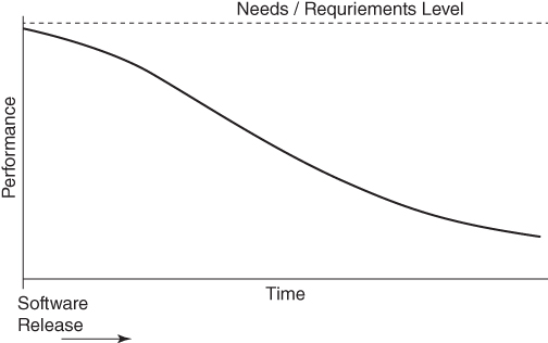
Figure 4.1 Software Decay Continuum
Another contributing factor toward the lack of software endurance is not a change in performance, but rather the changing needs and requirements of the customer. When software is planned and designed, its expected lifespan should be considered and established and, while code stability is beneficial to that lifespan, many data analytic projects are too dynamic to pin down indefinitely. For example, while building a complex ETL infrastructure to ingest data from international sources, I was already aware that the format of data streams would be changing in the upcoming months. But, rather than delay development, we released the initial version of the software on time so that the customer could receive business value sooner, with the understanding that an overhaul of the ingestion module would occur when third-party data structures were modified. Thus, the lifespan of the software was not diminished, but it did explicitly account for necessary maintenance.
In many cases, however, customers may not be able to predict shifts in needs or requirements. In another example, a separate ETL infrastructure was designed, developed, and released for production that featured once-daily data ingestion and reporting functionality. The customer naturally loved the SAS software so much that after a couple months of reliable operation, he decided that he wanted hourly—rather than daily—ingestion and reporting. A couple weeks later, while stakeholders were still discussing the feasibility of redesigning software to be faster and more efficient to meet this significantly higher threshold, a separate customer prioritized the addition of a separate data stream to the ETL software. Two more weeks passed, and the first customer then made a third request that the software reporting functionality should be updated.
In this classic example of software scope creep, because of these (and several other) change requests that were submitted by various customers, we decided to pool all new requirements over a period of three months, after which we designed, developed, tested, and released an overhauled version of the ETL infrastructure. During the requirements gathering and subsequent SDLC phases prior to release of the new version, however, the relative performance of the software continued to decline (as compared to the changing and increasing requirements that were being levied), despite the actual performance remaining stable and reliable. When the software was rereleased, software quality was again on par, as all functional and performance requirements were met.
Figure 4.2 demonstrates the performance of the initial software release, which decreases very slightly due to the expected decay continuum, but which is influenced more significantly by the continuous requirements being levied against the product. While this pattern continued after the first software upgrade, after the second software upgrade at six months, the software requirements were stabilized and performance was again acceptable.
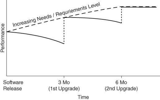
Figure 4.2 Increasing Requirements in Operational Phase
Software maintenance plays a pivotal role in software longevity in that software that is more maintainable is more readily modified and thus more likely to be maintained rather than scrapped. In the second example, we were able to modify the ETL software and release a new version (rather than entirely new software) because we had built software with maintainability principles such as flexibility and extensibility in mind. SAS software that lacks maintainability is more likely to more quickly fail to meet requirements as its performance and relative performance decrease in response to a shifting environment or shifting customer needs. This aspect is discussed in the “Stability Promoting Longevity” section in chapter 17, “Stability,” as well as in chapter 18, “Reusability.”
RELIABILITY IN THE SDLC
As the most commonly included performance attribute within requirements documentation, software reliability generally makes an appearance wherever technical requirements exist. Even where requirements are informal or implied, however, a general impression of the reliability that will be necessary for a software product should be established during software planning and design. Developers need to understand whether they're building a Mercedes or a Miata—in other words, will this software become an enduring cornerstone of SAS architecture, or a clunker that just needs to scrape by for a month or two? Both of these extremes—and everything in between—have their place in SAS development, but SAS practitioners must understand where on the reliability spectrum a software product lies before development commences.
Requiring Reliability
Because reliability is often mathematically defined within organizations and contractually defined in SLAs, reliability metrics are typically prioritized over other performance metrics. The type of reliability metrics defined will depend on software intent, heavily influenced by the expected software lifespan as well as the intended frequency of execution. Thus, the reliability objective will be very different for single-use SAS software as opposed to enduring software. Software developed within end-user development environments also may not require higher availability or reliability because SAS practitioners can perform maintenance or restart the software when necessary.
A SAS analytic program may only need to be run once to achieve a solution, after which the software is either empirically modified or archived for posterity and possible future auditing. Empirically developed software common in data analytic development environments is often produced and evolves through rapid, incremental development that chases some analytic thread toward a solution. Reliability in single-use software may be represented exclusively or predominantly by function rather than performance, for example, by demonstration that the correct solution and data products were generated. Neither longevity nor consistency is prioritized because software is not intended to be reused or rerun; availability is valued only insofar as it reflects a correct, available data product.
Other SAS software may specify a longer lifespan such as one year, but may not require frequent execution. For example, an ETL process may ingest data once a day or once per week, executing for some duration and then lying dormant until its next scheduled run. In these cases, reliability may be evaluated largely as a ratio of successful executions to total executions. For example, a process required to run once daily, seven days a week for a month would have 30 opportunities for success in September. If the software failed to complete or produced invalid results two of those days, this performance represents 28/30 or 93.3 percent reliability. Requirements can be this straightforward and simply state the reliability threshold that must be maintained by software.
Especially where software is consistently executed during its lifespan on some recurring schedule, another valuable metric is MTBF. If a SAS program runs once daily and the MTBF is four weeks, you can expect the software to choke about once a month. One consideration when establishing MTBF requirements is how to evaluate failures that can't be rectified before a next scheduled run. For example, if a daily SAS process fails two days in a row because it cannot be fixed immediately following the first failure, should the second failure be calculated into the MTBF calculation, even though it represents a continuation of the original unresolved error or defect? Thus, although fairly straightforward, the definition of MTBF in this example must resolve whether to include the second failure as a new event or a continuation of the first.
Still other SAS software may exhibit much higher execution frequency, such as systems that are constantly churning. Systems that offer continuous services, such as web servers, databases, or email providers, will often instead define reliability through availability metrics. For example, Amazon Web Services (AWS) guarantees “99.999% availability” for one of its server types, effectively stating that the AWS server will be down for no more than 5.5 minutes per year.15 Availability is measured not by the number or ratio of successful software executions but rather by the percentage of total time that a service or product is functional.
External Sources of Failure
Your SAS software fails, but it's not because of faulty code; an El Niño storm front took out the power to your block, bringing down not only the SAS server but the entire network. Your production SAS jobs that are scheduled to run every hour are obviously a lost cause for the day. But, while sitting in your dark cube twiddling your thumbs, a coworker mentions, “This is really going to kill our reliability stats for the month!” Should an act of God or other external factors discount the reliability of otherwise admirably performing SAS software? Moreover, what about that scheduled maintenance for next month to upgrade from SAS 9.3 to 9.4? How will that affect reliability performance required by your contract and collected through metrics?
One thing is clear—having this discussion literally in the dark, after a failure has occurred and brought down your system, is too late. Better late than never, though. External sources of failure, whether unplanned (such as power outages) or planned (such as required software upgrades), represent threats to reliability that should be discussed even if the decision is made to accept the risks they pose. These discussions and decisions typically occur at the team or organizational level rather than at the project level, and are thus conceptualized to occur outside (or before) the SDLC.
In some environments, the risk of failure due to external cause is essentially transferred from the developers or O&M team to the customer, in that the customer acknowledges and accepts that power outages, server outages, network outages, and other external sources of failure do occur and should not discount software reliability statistics. SAS practitioners should develop software that recovers from these failures using recoverability principles, but the practitioners aren't liable for securing backup generators, servers, or other hardware or infrastructure to prevent or mitigate external failures. For example, if a university's network connection drops, preventing researchers from accessing their SAS application, software, or data products, this likely would not be recorded as a software failure because it was beyond the control of the SAS practitioners.
Other environments are less permissive and require higher or high availability of at least the SAS server. SAS practitioners might be responsible for maintaining a duplicate server and data storage to support rapid system failover, but still would not be required to have backup power sources because that responsibility (and risk) would be borne at the organizational level. In this example, if the SAS server crashed and caused production software to fail, reliability metrics would reflect that failures had occurred because the SAS system failed to meet high availability requirements. After a power failure, however, reliability metrics would be undiminished because that risk would have been transferred to the customer or organization.
Reliability Artifacts
Reliability, more so than other quality characteristics, is benefited not only from quality code but also from external software artifacts, including a failure log and risk register. The risk register should be utilized throughout software development and testing; therefore, SAS practitioners and other stakeholders can use it to predict future software performance by assessing the cumulative nature, severity, and frequency of risks that exist. Thus, when software is released, developers should understand its strengths and weaknesses and effectively how reliably it should perform in production even before any failure metrics have been collected.
In software that will demand high reliability, requiring a risk register is a good first step to implement during software design to ensure that vulnerabilities are detected, documented, and discussed to calculate the ultimate risk that will be accepted when the software is released. Because software maintenance generally continues once software is operational, failures that may occur should be documented in a failure log but also should be included in the risk register if they exposed previously unknown or undocumented threats or vulnerabilities. Risk registers are described in the “Risk Register” section in chapter 1, “Introduction.”
The second reliability artifact, the failure log, is a necessity when the collection and measurement of reliability metrics are prescribed. Unlike the risk register, which only calculates theoretical risk of failure to software, the failure log records actual deviations from functional and performance requirements. It's often necessary to categorize failure by type or order them by severity. For example, if a SAS process is required to complete in less than 30 minutes but completes in 33 minutes one morning because of a slow network, this performance failure is worth recording, but might be significantly less detrimental than a functional failure in which the software abruptly terminates and produces no usable output. Reviewing, organizing, and analyzing failure patterns—rather than merely recording failures in a log—is critical to understanding and improving software reliability over its operational lifespan.
Reliability Growth Model
Imagine software that demonstrates a 10 percent failure rate—that is, one out of every ten times the software is executed, it incurs a functional or performance failure. If your Gmail crashed one out of ten times it was opened, or failed to send one out of ten emails, these functional failures would probably cause you to abandon the service in favor of an alternative email provider. Because reliability is so paramount to software operated by third-party users such as Gmail subscribers, companies such as Google attempt to deliver increasing performance over the lifespan of software, following the reliability growth model. For example, when a glitch occurs in Gmail and the box pops up asking if you'd like to submit data regarding the error, this is to facilitate Google's understanding of and ability to eliminate the exception or error in the future.
Reliability growth is “the improvement in reliability that results from correction of faults.”16 The reliability growth model describes software whose reliability increases over time, irrespective of other functional or performance changes that may occur. When a product is released, exceptions may be discovered that were not conceptualized during planning and design, or software defects may be discovered that were unknown during software testing. Thus, if software is maintained throughout its operation, and as defects are identified and resolved, reliability tends to increase asymptotically toward perfect availability over the software lifespan as depicted in Figure 4.3. Also note that because reliability and availability were prioritized into software design, the initial reliability at production was already 98 percent.

Figure 4.3 Reliability Growth Curve with Decreasing Failure Rate
In Figure 4.3, reliability continues to increase because stakeholders have prioritized its value within software requirements. Due to required maintenance also being prioritized to further higher levels of reliability, both the failure rates and MTBF will decrease over time. Thus, another way of conceptualizing the reliability growth curve is to imagine that the distance between failures tends to increase as sources of failure are mitigated or eliminated. If stakeholders decide to deprioritize maintenance, reliability will typically tend to stabilize, then diminish, following the decay continuum described in the earlier “Longevity” section.
In end-user development environments, reliability is often deprioritized in favor of greater functionality or in favor of a decreased software development period. Especially in data analytic development environments, SAS practitioners may be anxious to view software output so they can get to what we call “playtime”—turning data into information and knowledge. Moreover, because many SAS practitioners are end-user developers who are savvy software developers, when functional or performance failures occur, they can often immediately rerun, refactor, or revise the SAS software on the spot, avoiding painful change management processes that are necessary in some more traditional development environments. Thus, while end-user development will also typically follow the reliability growth curve, the initial reliability may be exceedingly less than exhibited by software applications intended for third-party users while the ultimate reliability achieved will also be significantly lower. Figure 4.4 demonstrates a typical end-user development reliability growth curve overlaying the traditional software growth curve observed in Figure 4.3.
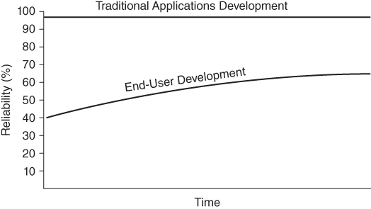
Figure 4.4 Traditional and End-User Development Reliability Growth Curves
Reliability growth models and decay continuums are useful in software planning and design because they can be used to model stakeholder expectations for software lifespan. If a customer wants an exaggeratedly high level of reliability or availability on day one of software release, that stakeholder must recognize the incredible amount of testing that will be required, not to mention beta releases to test the software with actual users. Even Gmail had beta releases while functionality and performance were still being tweaked. More appropriately, stakeholders can describe lower levels of reliability that might be acceptable in the first couple weeks or months of software operation, during which time reliability should advance toward higher reliability objectives as software errors and defects are eliminated through corrective maintenance.
Measuring Reliability
Reliability and availability metrics can have vastly different uses based on software intent, as well as how the risks of internal and external sources of failure are perceived. SAS practitioners must first understand which failure types contribute detrimentally toward reliability metrics and which (if any) represent accepted organizational risks such as power outages, network failures, or necessary software upgrades.
Table 4.1 demonstrates an extremely abbreviated failure log collected for SAS software from March through April. Reliability metrics are calculated from the failure log, as demonstrated in the remaining subsections of this chapter. This table is reprised in the “Measuring Recoverability” section in chapter 5, “Recoverability,” to demonstrate associated recoverability metrics.
Table 4.1 Sample Failure Log for SAS Software Run Daily for Two Months
| Error Number | Failure Date | Recovery Date | External/Internal | Severity | Description | Resolution |
| 1 | 3-16 3 PM | 3-17 9 AM | Ext | 1 | power outage | waited |
| 2 | 3-18 2 PM | 3-19 10 AM | Int | 1 | failure related to power outage | made more restorable |
| 3 | 3-25 10 AM | 3-25 11 AM | Ext | 1 | network outage | waited |
| 4 | 4-5 3 PM | 4-5 4 PM | Int | 1 | out of memory SAS error | restarted software |
| 5 | 4-22 9 AM | 4-22 1 PM | Int | 2 | minor data product HTML errors | modified HTML output |
Reliability can be complicated when it describes software that not only has failed but also must recover. For example, when the power fails, it must first be restored, after which the network and SAS server are restored, and finally SAS software is recovered. Software recovery is often captured separately in recovery metrics but the recovery period contributes to overall reliability when availability metrics are utilized. chapter 5, “Recoverability,” describes the interaction between these two intertwined dimensions of software quality.
Availability
As a measurement of reliability, availability is defined as “the degree to which a system or component is operational and accessible when required for use.”17 ISO goes on to clarify that it is “often expressed as a probability. Availability is usually expressed as a ratio of the time that the service is actually available for use by the business to the agreed service hours.” Availability is arguably the reliability metric most commonly utilized in software requirements documentation and SLAs.
Failure rate and MTBF each fail to describe reliability completely, because they typically are not weighted by the amount of time that software is failing and thus unavailable. In other words, did a subtle performance failure cause a momentary shudder in execution that was rectified in minutes, or did SAS practitioners have to rebuild the software over a grueling week of development during which time the software could not be run? Availability captures the percent of time that a system or software is functioning as compared to existing in a failed state. In doing so, availability incorporates not only reliability, but also the subcomponent of recoverability.
Availability metrics are most commonly implemented in software that requires higher or high availability. For example, if SAS analytic software is only run once per week, it only needs to be available for that one hour, so capturing availability could be difficult or pointless. But many SAS servers are required to be available 24×7, so even in environments for which no SAS software benefits from recording availability metrics, availability is the most common metric used to capture server reliability.
Where software is run frequently and consistently, availability can complement failure rate and MTBF because it incorporates the recovery period during which software is not operational. It primarily differs from the latter two metrics in that availability weights each failure by duration, while failure rate and MTBF do not. In essence, if a SAS job should execute once per hour but fails one Monday morning and cannot be restored until four hours later, this represents only one failure, even though four of the eight expected software executions for that day either failed or were skipped while subsequent maintenance was occurring. The failure rate would depict only one failure, while the availability would depict all four failures.
In Table 4.1, five software failures of external and internal cause are recorded in the failure log. If stakeholders have required that the software warrants redundant power, network, or other systems, then the team is liable for the risks posed by both internal and external vulnerabilities, and all five failures should be calculated into the availability metrics. In this case, if software is intended to be executed once per hour 24×7, the first entry results in 18 failures (because 18 executions were missed), the second entry represents 20 failures, and so forth. With 31 days in March, 30 days in April, and 24 hours per day, the software should have executed 1,464 times but, because it failed or was in a failed state 44 times, the software completed only 1,432 times. Thus, the availability is 1,420 / 1,464 or 96.99 percent.
Using the same failure log, consider that instead of running a 24×7 operation the SAS practitioners are responsible for lower availability software that operates 10×7 (8 AM to 6 PM, seven days a week). Thus, the first entry represents only four software failures (three on March 16 and one on March 17) rather than 18. Moreover, the total number of expected software executions drops to 610 or (61 days × 10 hours). Given this new paradigm, 16 failures occurred out of 610 software executions, so the availability is 594 / 610, or 97.38 percent. This underscores the importance of accurately determining when the software must be operational and when it can be allowed to be turned off or is undergoing maintenance.
As a final example, imagine a third team demonstrating the same software failure log, operating software from 8 AM to 6 PM seven days a week, but whose customer has stated that the SAS practitioners are not required to maintain the network, hardware, or other infrastructure. This is a common operational model in which the risk of failure of infrastructure components is effectively transferred to the customer or other IT teams. Where a power or network outage occurs, it's understood that the SAS practitioners are not liable, so these failures, while possibly recorded as “External” in the failure log, will not be included in reliability calculations.
When external causes of failure are removed from the reliability metrics calculations, only 11 software executions failed or could not execute because they were in a failed state. Thus, availability increases to 599/610 or 98.2 percent. This spread of availability rates in these three examples underscores the importance of adopting a risk management strategy before software release, as well as defining the scope of when and how often software is expected to execute.
Failure Rate
Failure rate is “the ratio of the number of failures of a given category to a given unit of measure.”18 The failure rate is a straightforward method of quantifying reliability, tracking the number of failures over time and within specified time periods. When failure rate is tracked longitudinally, the acceleration or deceleration rate of reliability moreover can demonstrate whether software performance is increasing or decreasing over time. For example, assessing the number of failures per week over a six-month period might demonstrate that while software is performing within specified reliability limits, its increasing failure rate signals that maintenance should be performed before the reliability threshold is exceeded.
Because failure rate can be calculated irrespective of the frequency of software execution or time interval between executions, it's extremely valuable when software is intended to be enduring but may not be run consistently or frequently. For example, if analytic software is only run the first week of the quarter but then lies dormant for three months, failure rate would be a preferred method to calculate its reliability because the metric does not take into account the dormant periods that complicate calculation of MTBF.
A limitation of failure rate is that it fails to account for the length of time that software is inoperable following a failure, the recovery period. Thus, to gain a more complete understanding of software's performance, it's often beneficial to calculate and track the recovery period as well. For example, when SAS software fails to meet performance requirements and completes in three hours rather than one, the performance failure should be documented, but no recovery period exists (because the software did not terminate with runtime errors or produce invalid results) so the software can be run again immediately. In other failure patterns, however, the software might be unavailable for an extended period for corrective maintenance following a failure. Especially in these cases, incorporation of recovery metrics can provide more context through which to interpret failure rates and severity.
In environments in which software is run consistently, such as software that is operated 24×7 in March and April, the failure rate will represent the unweighted availability. Thus, when the power outage caused the software to fail for 18 hours between March 16 and 17, this outage is treated as a single failure rather than 18 consecutive failures because it points to a single threat origin. Failure rate is easy to calculate, in this case five failures in two months or 2.5 failures per month. Because of the ease with which failure rate can be calculated, it is often tracked longitudinally to demonstrate acceleration or deceleration of failures, for instance three failures in January and two in February.
Because failure rate is simplistic, many teams choose to track failure rate by other qualitative characteristics in the failure log—often distinguishing liability such as internal versus external sources of failure. This could enable SAS practitioners and other stakeholders to demonstrate, for example, that software reliability might be increasing despite decreasing reliability in the SAS server or external infrastructure. Or, it might demonstrate that more significant functional failures are decreasing but performance failures are increasing. These metrics can enable stakeholders to prioritize maintenance to improve software performance. Thus, while simplistic and limited in some ways, failure rates gain power when combined with other qualitative metrics collected during and after software failure.
MTBF
Mean time between failures (MTBF) is “the expected or observed time between consecutive failures in a system or component.”19 It is measured by averaging the number of minutes, hours, or days between failures over a specified period. MTBF typically includes the failure period (i.e., recovery period) in which software is in a failed state and thus is measured from the incidence of one failure to the next. For example, if SAS software fails on a Friday, is restored to functionality on Tuesday, but fails again the next Friday, the MTBF is still seven days, representing the Friday-to-Friday span. Some definitions of MTBF conversely count from the point of recovery to the next failure, so it's important to define this metric. These two definitions are represented in Figure 4.5.

Figure 4.5 MTBF Competing Definitions, Inclusive and Exclusive of Recovery
MTBF is more sensitive to software execution frequency as well as the interval between software runs. For example, if SAS software is executed the first day of every month, and fails on March 1, the earliest it would again be executed (for production) is the April 1 execution, so the MTBF will always be at least one month. This one-month MTBF metric also fails to capture whether it took one day or three weeks to restore the software functionality, given that it was not required to be run again in production until April 1. For this reason, MTBF is best applied to software that runs frequently and consistently, but can also be incorporated with availability or recoverability metrics, both of which also take into account the duration of software failure in addition to its frequency.
Recall the five software failures recorded in the failure log in Table 4.1. The software warrants redundant power, network, and other systems, so the team is liable for the risks posed by both internal and external threats, and all five failures should be calculated into the MTBF calculations. In this case, if software is intended to be executed once per hour 24×7, the first failure occurs after 15 days and 15 hours (counting hours from 12:01 AM March 1). The second failure occurs 47 hours after the first; thus the first two metrics contributing to MTBF are 15.63 and 1.96 days and, continuing with this logic, the remaining time periods between failures are 6.83, 11.21, and 16.75 days, respectively. The final period from April 22 through May 1 is 8.63 days but isn't included because May 1 represents the end of the evaluation period rather than a failure. Thus, the MTBF for March and April is 52.38/5 or 10.48 days.
The inclusive MTBF definition will roughly approximate the total measurement period divided by the number of failures, in this case 61/5 or 12.2 days. In development environments that don't demand specificity, this can be an acceptable alternative to MTBF. A slightly more complex definition of MTBF excludes the recovery period from calculation. For example, if the power fails and brings down your SAS server, and cannot be revived for two days, reliability is not penalized for the duration that the system or software remains down. The calculations for inclusive and exclusive MTBF are compared in Table 4.2.
Table 4.2 Inclusive versus Exclusive MTBF Calculations
| Error Number | Failure Date | Restore Date | Inclusive MTBF | Exclusive MTBF |
| 1 | 3-16 3 PM | 3-17 9 AM | 15.63 | 15.63 |
| 2 | 3-18 2 PM | 3-19 10 AM | 1.96 | 1.21 |
| 3 | 3-25 10 AM | 3-25 11 AM | 6.83 | 6 |
| 4 | 4-5 3 PM | 4-5 4 PM | 11.21 | 11.67 |
| 5 | 4-22 9 AM | 4-22 1 PM | 16.75 | 16.71 |
| MTBF | 10.48 | 10.14 |
While the difference in the calculated metrics is subtle and can seem like splitting hairs, the exclusive MTBF eliminates time spent restoring software. The calculation for exclusive MTBF is more complex because both failure and recovery points must be recorded. A benefit of this method, however, is it more accurately demonstrates time that the software is actually functioning, rather than also incorporating time that the software is being restored and possibly even modified with corrective or emergency maintenance.
In other words, stakeholders assessing the performance of software may be asking the basic question, “How long was your software running this time before it failed?” In posing the question in this manner, stakeholders are requesting the exclusive MTBF—measured from the last recovery point to current failure—because they are not concerned with how long it took to modify and recover software following the last failure. Whichever method is selected—internal or external MTBF—it should be defined leaving no room for ambiguity or misinterpretation.
WHAT'S NEXT?
Reliability is the most critical dynamic performance attribute and, as described, incorporates availability, which measures performance against failure. For this reason, high availability requires swift software recovery, facilitated by recoverability principles. In the next chapter, recoverability—a subcomponent of reliability in the ISO software product quality model—is introduced and demonstrated.