
Chapter 5
Recoverability
I'd worn the same pair of button-fly 505 Levi's for a month while backpacking through Central America and, aside from some pupusa stains and the subtle accumulation of chicken bus grime, they'd been exceedingly durable and reliable.
Busing and hitchhiking in pickup beds through Columbian FARC country, I'd finally arrived at San Andrés de Pisimbalá, a remote, mountainous pueblo bordering the Tierradentro archaeological and UNESCO World Heritage Site. Remote and inaccessible except by horseback, the seldom-seen Tierradentro features pre-Columbian tombs carved into hilltops with 7th-century ceramics and polychromatic paintings in situ.
Having serendipitously met my guide's wife while hitchhiking the gravelly road to San Andrés, I saddled up and followed Pedro on horseback, dismounting at numerous tombs to descend down rock-hewn spiral steps into spaciously carved caverns and indescribable antiquity. As the day wore on and the equatorial sun beat down, I was thankful for the cool breeze but, while dismounting at one site, the breeze suddenly intensified and I realized that amid the jolting, jarring hours on horseback I had completely ripped out the crotch of my Levi's. ¡Ay caramba!
The front-to-rear tear was catastrophic and career-ending for the Levi's; the guide and his wife were amused when, back at the hostel, I learned that she could not repair the rip with a patch. I'd be in Quito, Ecuador, in a couple days, so I was resolved to modesty until then as I left San Andrés and continued onward.
Having lived in Ecuador previously, I reached out to Andres, a friend in Quito who, despite laughing at my crotchless travels, was happy to assist with my latest backpacking debacle. We searched for hours, going from mall to mall and, even with my interpreter, it took four hours to find a single pair of jeans that I could squeeze my gringo-sized body into.
At long last, Tommy Hilfiger came to the rescue; despite a ridiculous price of US$124, the jeans have been equally reliable, surviving South America and beyond.

If you start with a quality product—such as Levi's or Tommy Hilfiger jeans—you'll be less concerned with failure because the product is inherently more reliable and durable. But even 505s or extremely reliable software will fail at some point, and when this occurs, recoverability principles dictate how quickly recovery can occur.
My jeans theoretically could have been patched, but they were five years old, had had a good life, and were becoming threadbare elsewhere. Software, however, doesn't weaken or wizen over time, so failure typically doesn't denote end of product life. For example, when a hapless SAS administrator accidentally turns off the server, causing all SAS jobs to fail, the SAS server can be turned on again and the SAS jobs will continue to execute.
But recovery can be delayed where infrastructure outside the control of SAS practitioners has failed, such as power or network failures. In the remote Colombian mountainside, no amount of effort or time could have repaired or replaced my torn jeans—I could only close my legs and be patient while transiting to Quito. SAS practitioners, too, will encounter external causes of software failure that cannot be remedied and must be waited out; recoverability principles cannot lessen these delays.
With infrastructure restored, however, or in the case of failures that were programmatic in nature, the software should be able to be restarted easily and efficiently, but sometimes that is not the case. As with driving around Quito for hours, running from one mall to the next, developers can incur inefficiency and tremendous expense of time if software has to be jumpstarted through convoluted procedures or emergency maintenance to restore functionality.
Inefficiency is especially likely when failure was not predicted and no recovery strategy exists, or recovery efforts compete against other objectives. I knew I would eventually find jeans in Quito—at over 2.5 million Quiteños strong, plenty of shopping venues exist—but I didn't know the malls, the brands, the sizes, or the language, and all of these factors contributed to inefficient shopping. When software fails unexpectedly on a Tuesday, developers may have to spring into action, suppressing other activities and inefficiently prioritizing maintenance over scheduled work.
Recoverability principles thus seek to increase the overall reliability and availability of software by minimizing the amount of time required to restore software and data products following a failure.
DEFINING RECOVERABILITY
Recoverability is “the degree to which the software product can re-establish a specified level of performance and recover the data directly affected in the case of a failure”1 In the case of failed software, the failure could have been caused by the SAS software itself or by any element of its infrastructure, such as the SAS application, SAS server, network, hardware, or even power supply. Recoverability is a critical component of reliability, especially in high-availability systems that measure time in a failed state against operational time.
Software recovery cannot prevent external sources of failure such as power outages from felling SAS software, but when the cause of the failure has been eliminated and the SAS server is operational, recoverability principles minimize the amount of time required to restore SAS software and, in some cases, the resultant SAS data products. Software recoverability principles follow the TEACH mnemonic: software recovery should be timely, efficient, autonomous, constant, and harmless.
In other cases, software fails because of internal causes, such as software defects or other errors that require corrective or adaptive maintenance. Software must be modified before it can be restored, which can be both time consuming and risky when unplanned emergency maintenance must be performed. Maintainability principles demonstrated throughout chapter 13, “Maintainability,” include best practices to support efficient and effective modification. When emergency maintenance occurs after a failure, however, this maintenance contributes to the recovery period and detracts from overall software reliability. Therefore, where software modification must occur during recovery operations, maintainability principles as much as recoverability principles will guide software recovery. This chapter demonstrates TEACH principles across discrete phases of the recovery period that follow software from failure to recovery.
RECOVERABILITY TOWARD RELIABILITY
Many products, such as jeans, must be disposed of when they fail because failure represents end of product life or, in less extreme cases, the need to at least repair the product. In this sense, the mean time to recovery (MTTR) for software may in some environments be referenced instead as mean time to repair, reflecting terminology typically reserved for physical products. In physical products, mean time to failure (MTTF) describes the product life before it fails, typically with the expectation that the product will be discarded at failure. In describing software, however, mean time between failures (MTBF) rather than MTTF is used because software failure is presumed not to denote end of life but rather the start of the recovery period, after which software can continue operation.
In many cases, a performance failure may cause software to fail in the sense that it fails to meet performance requirements, but software neither terminates nor produces invalid data or data products. For example, SAS software that occasionally completes too slowly can cause performance failures when execution time exceeds technical requirements. Unless software is terminated after a performance failure to allow SAS practitioners to perform corrective maintenance, no recovery period or recovery exists, so recoverability principles are irrelevant. For this reason, failure logs—demonstrated in the “Failure Log” section in chapter 4, “Reliability”—typically distinguish functional from performance failures so they can be tracked independently.
Therefore, recoverability represents an aspect of quality that, while critical to software development environments, is uncommon in most physical product types. Figure 5.1 compares MTTF patterns for a physical product like a pair of jeans to MTBF patterns for software. Note that no recovery period exists for the software experiencing only performance failures from slowed execution.
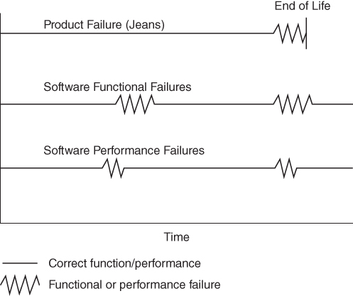
Figure 5.1 Comparing MTTF and MTBF
Described as a subcomponent of reliability in the International Organization for Standardization (ISO) software product quality model, recoverability contributes to reliability because it minimizes the recovery period during which software is in a failed state, providing no or limited business value. Achieving reliable software is the most crucial step in maximizing software availability; code that doesn't fail in the first place won't need to recover. But because software failure is an inevitability, software that requires high reliability and availability must also inherently espouse recoverability principles to facilitate these goals.
Environmental, network, system, data, and other external issues can cause lapses in connectivity, memory errors, and other failures that result in unavoidable program termination. Planned outages, including upgrades and modifications to SAS software, its infrastructure, network, and hardware also require halting operational SAS programs. While recoverability reflects the ability to restore functionality or availability of a system or software following a failure or planned outage, recovery represents the state of restored functionality or availability, and the recovery period the time and effort required to restore the system or software.
The “Reliability Growth Model” described in chapter 4, “Reliability,” demonstrates the increasing reliability of software that is appropriately maintained over time. Figure 5.2 demonstrates the decreasing failure rates and increasing MTBF associated with the reliability growth curve, representing that software reliability and maintenance have been prioritized. In this example, however, rather than merely indicating when each failure occurred, the duration of the failure also is shown.

Figure 5.2 MTBF Influencing Reliability Growth Curve
While the reliability growth curve demonstrates decreasing failure rates, it says nothing about the recovery period or duration of each failure. Thus, while higher availability and decreased failure rates can be achieved simply by following the reliability growth curve, the recoverability growth curve shows that availability can be further increased by decreasing the recovery period through the implementation of recoverability principles and phases.
Recoverability Growth Model
The recoverability growth model is a corollary to the reliability growth model, effectively demonstrating that where recoverability principles are prioritized in software, the software recovery should decrease asymptotically over time toward theorized automatic, immediate recovery. The recoverability growth curve is demonstrated in Figure 5.3, in which lower recoverability denotes longer recovery periods and higher recoverability denotes shorter recovery periods.
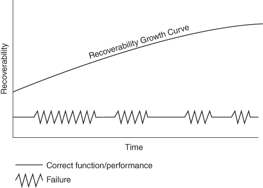
Figure 5.3 Recoverability Growth Curve with Decreasing Recovery Period
The recoverability growth curve often occurs in conjunction with the reliability growth curve. Thus, as SAS practitioners hone software and make it more resilient and robust, they often additionally seek to improve recovery because they learn ways to eliminate or make recovery phases more efficient. The recoverability curve is irrespective of the reliability curve, as Figure 5.4 demonstrates both the combined and individual effects of reliability and recoverability in relation to each other.
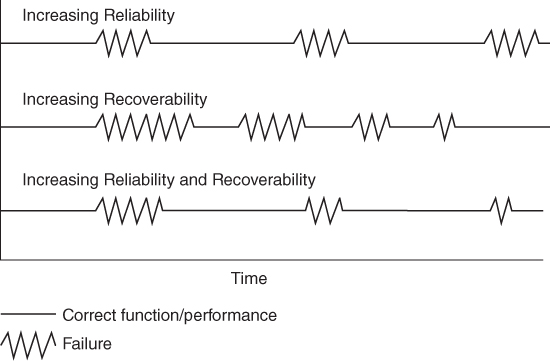
Figure 5.4 Interaction of Reliability and Recoverability
Availability is demonstrated by the percent of time that software is not in a failed state. As demonstrated in Figure 5.4, while the reliability growth curve and recoverability growth curve can occur separately over the software lifespan, the highest software availability occurs when both reliability and recoverability are maximized.
RECOVERABILITY MATRIX
In 2015, I introduced the Recoverability Matrix, which describes guiding principles that facilitate software recoverability as well as discrete phases that software passes through en route to recovery.7 By incorporating these principles into code, SAS practitioners can facilitate code that minimizes and often eliminates phases entirely, thus tremendously improving the recovery experience.
Recoverability principles follow the TEACH mnemonic and state that software recovery should be:
- Timely—The recovery period should be minimized to maximize availability.
- Efficient—Recovery should be efficient, including an efficient use of software processing (i.e., system resources) as well as developer resources if maintenance is required during recovery.
- Autonomous—From failure detection to functional resumption, recovery should minimize or eliminate human interaction and recover in an intelligent, automated manner.
- Constant—Quick-fixes, jumpstarts, and one-time code bandages that facilitate recovery should be avoided in lieu of strategic, repeatable, enduring solutions.
- Harmless—The recovery process should not damage the data products or other aspects of the environment.
Each of these principles should be demonstrated throughout the following discrete phases that can occur during the recovery period after failure has been detected. The SPICIER mnemonic describes recovery phases that may exist but, in many cases, should be minimized or eliminated through recoverability principles.
- Stop Program—Because failure does not necessarily denote that software has stopped running, the software may need to be stopped.
- Investigation—Gather information about the source, cause, duration, impact, potential remedies, and other aspects of the failure.
- Cleanup—Remove faulty data, data products, or other results that may have been erroneously created due to the failure.
- Internal issues—Corrective, adaptive, or emergency maintenance may be required to restore software functionality.
- External issues—Issues beyond the immediate control of SAS practitioners may have caused the failure, but these may need to be researched or have quality controls applied to improve or automate future failure detection.
- Rerun code—The final phase in the recovery period and, after especially heinous failures that have crippled critical infrastructure, the point at which SAS developers tap that keg and finally celebrate.
TEACH RECOVERABILITY PRINCIPLES
An ideal recovery is timely, efficient, autonomous, constant, and harmless—tightly intertwined principles depicted through the TEACH mnemonic. Timeliness reflects the speed with which the recovery occurs, including discovery of the failure, how long it takes to restart software, and how long it takes to surpass the point of original failure within the code. Efficiency demonstrates code that does not require excessive processing power or developer effort, the latter of which can be eliminated through autonomous code. Autonomy reflects software that identifies failure, terminates automatically if necessary, and can be restarted with the push of a button without further developer intervention. Software constancy demonstrates that a recovery strategy is enduring, not an expedient “quick fix” that will need to be later improved or undone. Harmless software should both fail and recover without damaging its environment, such as causing other processes to fail or producing invalid data products.
Timely
Just as software speed is often used as a proxy to represent overall software performance, timeliness of recovery often acts as a proxy for other recoverability principles. When software recovery occurs quickly or instantaneously, the assumption is that other principles must have been followed. Thus, other recoverability principles often are not prioritized unless recoverability or reliability performance metrics are not being achieved.
At a higher level, recovery is viewed as a single event that restores functionality and terminates the recovery period. The RTO, if present in requirements, specifies the time period within which the average recovery must occur. Thus, the actual MTTR achieved over time should always be less than the RTO although individual recovery periods may exceed the RTO. In more restrictive environments, the RTO is interpreted as a maximum recovery period that no single recovery period should ever exceed. In this latter sense, implementation of the RTO more closely approximates the MTD. Figure 5.5 demonstrates six software failures whose recovery periods have been measured and recorded against recoverability requirements. While the MTTR fell below the RTO, one failure did take longer to recover than the RTO, which represents a performance failure. All recoveries did occur far below the MTD that stakeholders had established.

Figure 5.5 MTTR, RTO, and MTD
In the case of Figure 5.5, in which the RTO was not achieved because of one performance failure, attention should shift from higher- to lower-level recovery, including discrete phases that can occur during the recovery period. For example, SAS practitioners might discover that during the single failure, the cleanup phase of recovery took longer because invalid data products had been created and had to be corrected. Thus, in seeking to deliver more consistent recovery in the future, timeliness of the SAS software could be improved by investigating and improving individual phases of recovery.
Efficient
Efficiency can be represented by the effort or resources that a person or process must expend to facilitate software recovery. For example, an inexperienced SAS practitioner who is unfamiliar with specific software would be less efficient in investigating and remedying a failure than a more experienced developer who had authored the software. Code that is difficult to read or poorly documented can also unnecessarily delay recovery because it is not intuitive and thus more difficult to maintain and modify. A failure that requires substantial cleanup of the SAS system because the code produced spurious data, metadata, or data products can also be an inefficient use of a developer's time, because that cleanup could likely have been eliminated or could have occurred automatically, were more rigorous software development practices enforced. While software failure is never a pleasant experience, through proactive design and development, developers can ensure that their time is well utilized during the recovery period.
Development time, however, is not the only resource that must be taken into account. Software itself should recover efficiently, demonstrating a competent use of system resources and execution time. If SAS code fails to recognize that an internal failure has occurred and the failure goes unnoticed for hours or days, this is an inefficient use of the SAS processor, which was effectively churning without purpose for days while producing invalid results that must be reproduced after recovery. When a program must be rerun at the close of the recovery period, efficient code should also intelligently bypass any unnecessary steps. Checkpoints can demonstrate code modules that have completed successfully prior to failure, thus enabling process flow to skip these and proceed directly to the point of failure. This technique is demonstrated in the “Recovering with Checkpoints” section later in the chapter.
Autonomous
Autonomy typically includes and supersedes automation, specifying that a system is not only free from human interaction but also able to make decisions intelligently. Fuzzy logic SAS routines can guide processes to detect failure automatically and, based on metadata collected about the failure, to recover automatically in many cases. Process metrics collected during software failure can demonstrate the type and location of exceptions or errors, especially if they can be compared with baseline metrics that demonstrate previous process success. By predicting and detecting specific error types in exception handling routines, software can often terminate gracefully, thus setting the stage for a cleaner, more efficient recovery.
Consider a SAS process that fails because a required input data set is not available when the software is run. Autonomous recovery begs the question, “What steps would a skilled SAS practitioner follow in this situation?” and recreates this logic in software. For example, when alerted to the exception of the missing data set, the software might automatically send an email to stakeholders to inform them while entering a busy-waiting loop for a number of hours to give developers the chance to rectify the missing data set. After a parameterized amount of time, the software could gracefully terminate if the data set still could not be located. However, if stakeholders were able to restore the availability of the input data set, recovery could occur quickly and efficiently without a single runtime error.
This scenario underscores the importance of autonomy and automation throughout all recovery phases. For example, the obvious bottleneck in the proposed solution is the intervention of SAS practitioners, who must first receive an email and then perform some action. A single bottleneck that relies on human interaction can cause significant delays in recovery systems that are otherwise streamlined and automated, but in many cases it's unrealistic to expect an automated process to transfer the necessary data set to its expected location, so total automation may not be achievable. Notwithstanding, even adding processes that automatically detect and communicate software failures will provide a tremendous advantage for software recovery.
Constant
Constancy or consistency reflects stability in code over time, including the manner in which software is executed and the steps taken to revive software following failure. Stable software should be dynamic enough to determine how and where to restart after a failure. Thus, rather than highlighting sections of code to be run manually or creating quick fixes to be used to jumpstart code, developers should be able to run the same code in its entirety every time—whether following a successful or failed execution. Temporary solutions that can revive and run software today may be timely but, if they introduce new defects or technical debt that must be dealt with tomorrow, this added cost is typically not worthwhile.
For example, suppose that a serialized extract-transform-load (ETL) process is executing that ingests and transforms 20 SAS data sets in series. If the process fails on the 16th data set after successfully processing 15 data sets, some SAS practitioners might be tempted to rerun the software with manual modifications that specify that the software should start at the 16th rather than the 1st data set. This type of rogue emergency maintenance is abhorred in production software and should be avoided at all cost! Another tempting but terrible idea would be to rerun the software in its entirety, thus needlessly reprocessing the first 15 data sets and obviously violating the principles that recovery should be timely and efficient.
A consistent software solution, on the other hand, might instead consult a control table to interrogate performance metrics, which would demonstrate that the first 15 data sets had been processed, thus dynamically enabling the software to begin processing on the 16th data set rather than the 1st. As a result, software can remain constant by implementing dynamic processes that effectively utilize checkpoints, thus eliminating the poor practices of rogue software modification or redundant processing. This revised solution, which dynamically assesses past successes and failures of the software, can be utilized to execute software every time it is run, regardless of whether the previous execution succeeded or failed. The benefits of consistent, stable software are demonstrated throughout chapter 17, “Stability.”
Harmless
When harmless software fails, it should not adversely affect its environment, such as by producing faulty, incomplete, corrupt, or otherwise invalid data, metadata, data products, or output. Harmless code should automatically detect a failure when it occurs and handle it in a predictable, responsible manner, because only through predictability comes the assurance that dependent processes and data products are not negatively affected. In most cases, it is far more desirable to have data products that are unavailable or delayed (due to detected failure) than those that are dead wrong (due to undetected failure).
Not only failure but also recovery should be harmless, so the environment should not be altered unfavorably in an attempt to restore functionality. For example, if a developer modifies SAS library names in a production environment as an expedient solution to rerun code that has failed (because it erroneously referenced library names in the development environment), this could cause unrelated processes to fail. Another scenario often occurs in which software fails because of an exception or error within a macro shared by the development team. The temptation may exist to alter the macro so that it works in the current software that is failing, but if this modified macro is reused in other production software, the change cannot be made until the implications of the proposed modification are understood. A software reuse library, demonstrated in the “Reuse Library” section in chapter 18, “Reusability,” can facilitate an awareness of code use and reuse and ultimately backward compatibility when maintenance is required.
SPICIER RECOVERABILITY STEPS
While TEACH depicts recoverability principles that should be applied during software design and development, the SPICIER mnemonic identifies specific phases of the recovery period, each of which can be optimized through recoverability principles. In many cases, many if not all recovery steps can be automated, and some steps, such as cleanup, should often be eliminated in production software.
Stop Program
Failure comes in all shapes and sizes but does not necessarily denote program termination or even that runtime errors were produced. Failure can occur not only when software produces runtime errors or terminates abruptly, but also when it enters a deadlock or infinite loop, or continues to execute albeit producing invalid data, data products, or other output. A common goal of exception handling routines is to channelize software outcome toward two distinct paths, the happy trail and the fail-safe path.
The happy trail (or happy path) is the journey that software takes from execution to successful completion and delivery of full business value. When exceptions or errors are encountered, however, robust software aims to get back on the happy trail toward restoration of full or partial functionality. In other words, something bad happens during execution, but the software limps along or is fully restored, ultimately delivering either full or partial business value. Software that lacks robustness will still have an underlying happy trail, but once exceptions occur, no methods exist to rejoin that trail, so the software can only fail.
The fail-safe path is the alternative path in which software fails gracefully due to exceptions or errors that were encountered. Functionality halts and no or minimal business value is delivered, but the environment is undamaged and remains secure. An example of unsecure termination would be abruptly and manually aborting SAS software because invalid output had been detected by analysts. Secure termination, on the other hand, might automatically detect the abnormalities in output, update a control table to reflect the exception or error, and instruct SAS to terminate. Thus, automatic software termination must always begin with automatic failure detection.
Although production software should fail gracefully when errors are encountered, if an unexpected error is encountered for the first time, software may fail in an unsafe or unpredictable manner. In these cases, if software is still executing but errors have been detected, it must be terminated manually. For example, if an ETL program that performs daily data ingestion requires tables to have 40 fields, but on Monday it encounters a table that has only 37 fields, the process flow should be robust enough to detect this exception automatically. Business rules would direct the exception handling, but might include immediate program termination with notification to stakeholders, as well as preventing dependent processes from executing. If the system is not robust and does not detect the 37-field discrepancy, subsequent code could continue to execute and create invalid results, even if no runtime errors were produced.
Timely, efficient, and autonomous termination can often be achieved through exception handling routines that detect exceptions and runtime errors and provide graceful program termination. For example, the following SAS output demonstrates an error that is produced when the file Ghost does not exist:
data temp;
   set ghost;
ERROR: File WORK.GHOST.DATA does not exist.
run;
NOTE: The SAS System stopped processing this step because of errors.
WARNING: The data set WORK.TEMP may be incomplete. When this step was stopped there were 0 observations and 0 variables.
WARNING: data set WORK.TEMP was not replaced because this step was stopped.
%put &SYSCC;
1012
Testing the automatic macro variable &SYSCC after each procedure, DATA step, or other module offers one way to determine programmatically whether a runtime error occurred and can be utilized to alter program flow dynamically thereafter. The use of SAS automatic macro variables for use in exception detection and handling is described extensively in chapter 3, “Communication,” and in the “Exception Handling” section in chapter 6, “Robustness.”
Software failures, however, are not always signaled by runtime errors. The 37-field data set described earlier was structurally unsound and would produce invalid results yet possibly yield no obvious runtime errors. As another example, if the following code is run after the previous code, it runs without producing a runtime error but is still considered to have failed because an empty data set is produced:
data temp2;
   set temp;
run;
NOTE: There were 0 observations read from the data set WORK.TEMP.
NOTE: The data set WORK.TEMP2 has 0 observations and 0 variables.
It turns out that despite encountering an error, the first DATA step creates the Temp data set even though it has zero observations and zero variables. Thus, the second DATA step executes without warning or runtime error, despite having invalid input. In testing for conditions that should direct a program to abort, software must examine more than warning and error codes and must validate that business rules and prerequisite conditions are met. The following code first tests to ensure that the data set contains at least one observation and, if that requirement is not met, the %RETURN statement causes the macro to abort:
%macro validate(dsn=);
%global nobs;
%let nobs=;
data _null_;
   call symput('nobs',nobs);
   stop;
   set &dsn nobs=nobs;
run;
%mend;
* inside some parent macro;
%validate(dsn=work.temp);
%if &nobs=0 %then %return;
* else continue processing;
Despite diligence in software exception management, on occasion software will still need to be terminated manually. Terminating software manually reinforces the reality that software can fail inexplicably at any line of code. The hapless developer who trips over a cable and disconnects his machine from the server could do so while any line of code is executing. Recoverability requires developers to espouse this mind-set and ask themselves, after every line of code, “What will happen if my code fails here?” This mind-set reflects that code should always fail safe, in a harmless, predictable manner. This aspect is discussed more fully in the “Cleanup” section later in this chapter, because code that fails safe and is harmless will not require cleanup, thus avoiding this sometimes agonizing aspect of the recovery period.
Investigation
Where program termination has resulted from a scheduled outage due to maintenance or other program modification, this step won't be necessary because failure was planned. But in cases in which unplanned failure has occurred in production software, stakeholders will be clamoring not only for immediate restoration but also for answers. From a risk management perspective, higher-level stakeholders are often not concerned with great technical detail, but rather with more substantive facts surrounding the failure, such as “What caused this failure?” and “Will it happen again?” A best practice is to record these and other qualitative information about the failure in the failure log, as discussed in the “Qualitative Measures of Failure” section in chapter 4, “Reliability.”
Log files are a recommended best practice for production software because they can help validate program success through a baseline (i.e., clean) log and facilitate the identification of runtime or logic errors. When the failure source is captured in the log file and through continuous quality improvement (CQI), developers are able to refactor code to improve robustness, eliminating one failure at a time from occurring in the future, as depicted in the “Reliability Growth Model” section in chapter 4, “Reliability.” In other cases, the log file may exist but may not contain sufficient information to debug code. This also occurs when errors in business rules or logic may not be immediately perceived, resulting in the deletion of relevant log files before they can be analyzed. When this occurs, the code may require extensive debugging and test runs to reproduce and recapture the failure with sufficient information to understand the underlying defect or error.
Maintenance of a risk register is another best practice for production software because it describes known defects, faulty logic, and other software vulnerabilities that can potentially cause program failure. After encountering a failure, SAS practitioners can turn to the risk register to investigate whether associated threats and vulnerabilities had been identified for the failure and, in many cases, whether maintenance or solutions had been proposed. This is not to suggest that action will be taken once the source of failure is identified, but elucidation of the vulnerability is critical to assessing risk in reliable software. Use of the risk register is discussed in “The Risk Register” section in chapter 1, “Introduction.”
Cleanup
After investigation of a failure, the next step is either to rerun the software or perform maintenance if necessary. Especially in cases in which no defect exists and software failed due to an external threat such as a power outage, software should be able to be restarted immediately without further intervention. This pushbutton simplicity can be thwarted, however, when failures produce wreckage in the form of invalid data products—including data sets, metadata, control tables, reports, or other output. The principle that recovery be harmless dictates that carnage not be produced by production software; thus the site of failed software should not resemble an accident scene, with bits of bumpers, broken glass, and the fetid stench of motor oil and transmission fluid seeping into the asphalt.
Cleanup is typically required when some module or process started and did not complete, but left the landscape nevertheless altered. Some examples include:
- A data set is repeatedly modified through successive processes. After the failed process, the original data set is no longer available in its original format because some (but not all) transformations have occurred.
- A data set was locked for use with a shared or exclusive lock, after which the process failed before the data set could be unlocked. The data set may be unavailable for future use until the SAS session is terminated.
- The structure or content of a directory is modified, after which a failure occurs. For example, if raw data files were moved from an Original folder to a Processed folder, they may need to be moved back if the ingestion process was later demonstrated to have failed.
- A control table was updated to reflect that a process started but, because the process failed, the control table may never have been updated with this information. In many cases, SAS practitioners must manually edit the control table to remove these data, which can be risky when control tables contain months of precious, historical performance metrics and other metadata.
The first example often occurs in serialized ETL processes, in which each DATA step or procedure is dependent on the previous one. A DATA step may undergo successive transformations that, to save disk space or avoid complexity, are performed on the same data set without modifying its name. In the following example, the Final data set seems to indicate some finality, but instead is modified several times. Thus, if the code fails, it may be difficult to determine which transformations have occurred successfully (and should not be repeated during recovery). Moreover, where transformations permanently delete, modify, or overwrite data, it may be impossible to recreate the initial data set if necessary:
data final;
   length char1 $15;
   char1='taco';
run;
data final;
   set final;
   length char2 $15;
   char2='chimichanga';
run;
data final;
   set final;
   length char3 $15;
   if char1='taco' then char3='flauta'; * theoretical failure    occurs here;
run;
Cleanup can also be required when explicit locks are not cleared because software fails before this can be done. Explicit locks are beneficial because they can ensure that a data set will be available before software attempts to utilize it. When an exception is encountered in which the data set is either in use or missing, the process can enter a busy-waiting cycle to wait for access or it can fail gracefully, thus avoiding runtime errors. The LOCK statement explicitly invokes an exclusive lock and was historically used in busy-waiting cycles, but its use has been deprecated (outside of the SAS/SHARE environment), as discussed in the “&SYSLCKRC” section in chapter 3, “Communications.” Rather, FOPEN can be used to secure an exclusive lock on a file or data set, and OPEN to secure a shared lock. These functions, however, require the FCLOSE and CLOSE functions, respectively, to ensure file streams are closed, as demonstrated in the “Closing Data Streams” section in chapter 11, “Security.”
Another example of cleanup describes changes in folder structure or content that often occur as part of an ETL process. Consider an ETL process that I once inherited from another SAS practitioner. Raw text files were continuously deposited into a folder Inbox and, once a day, the ETL process would first create a folder named with the current date, then copy all accumulated text files from Inbox to the new folder, then ingest and process the files. The software was fairly reliable but, when it did fail, it failed miserably and required extensive cleanup.
When the text files were copied from Inbox to the respective daily folder, this process created an index that was later used to ingest each file. So, if the process failed sometime after files had been copied during ingestion, when the software was restarted, no files would be in the Inbox, so no new index would be created. Thus, to restart the software after a failure, the files had to be moved back to the Inbox, the index deleted, and a separate control table updated to reflect that the process was being rerun. While moving data sets or other files on a server can be a regular part of data maintenance and should be automated to the extent possible, SAS practitioners must also consider the implications of whether those actions and automation could cause later cleanup if software were to fail.
In all cases, SAS practitioners should strive to design and develop processes that require no cleanup, which not only can be costly but also can introduce the likelihood of further errors. Having to copy or rename files, modify data sets, edit control tables, or unlock data sets manually is risky business and should be avoided on production software.
Internal Issues
Once software has failed and stopped, the cause and potential remedies have been investigated, and any necessary cleanup has occurred, the next step is often to rerun the software. For example, this occurs when the software failed because of a power or server outage and no software maintenance is necessary. In the most straightforward failures, internal issues do not exist, and this phase is skipped entirely.
But what happens when the power fails and software isn't able to start immediately? Perhaps extensive cleanup of the landscape is required, or numerous software processes that had already completed need to be rerun, causing inefficiency. These all represent internal issues that should be corrected if recoverability has been prioritized, despite the actual failure occurring due to external causes. Thus, internal issues primarily describe corrective, emergency, or adaptive maintenance that must be performed on software either to restore functionality or to improve recoverability when future failures occur.
Some internal issues may not require software maintenance but may require SAS practitioners to resolve other issues in their environment. For example, if ETL software fails because a data set is locked by another process, the second process may need to be stopped (or waited for) so that the ETL software can be rerun after the data set is made available. In a similar example, memory-intensive SAS software can cause an out-of-memory failure, sometimes in the software itself and sometimes in other SAS software running concurrently on the server. Thus, when memory failures occur, other processes may need to be stopped (or waited for) so that the primary software can be restored and run with sufficient memory.
But if vulnerabilities or defects were identified in the code, or if developers or other stakeholders have decided that the recoverability or performance needs to be improved through maintenance, then the software itself must be modified in this phase. Maintenance types such as adaptive, perfective, corrective, and emergency are described in chapter 13, “Maintainability,” and by embracing maintainability principles in software design, maintenance can be performed efficiently after a failure, minimizing the recovery period.
External Issues
External issues reflect anything that stands between SAS practitioners and the recovery of their software—anything over which they have no control. The cause of failure may have been external, such as a failed connection to an external database administered by a third party. In this case, SAS practitioners would begin making phone calls to attempt to ascertain the cause of the failure and its expected duration. In many cases when an external cause is identified during investigation, a development team can only sit around and wait for the external circumstance to be rectified.
So what else can SAS practitioners do once software has crashed while they're twiddling their thumbs waiting for someone to restore a data stream? My team once lost a critical data connection to Afghanistan, and team members kept asking one of our developers, “Is the connection up yet? Do we have data?” And each time he was asked, the developer would disappear to his desk and rerun the software, producing hundreds of runtime errors that demonstrated not only the single exception—the broken data stream—but also cascading failures resultant from a total lack of exception handling. As it turns out, when external issues are preventing software from executing, this is the perfect time to build data connection listeners and other quality controls that test negative environmental states.
A negative state could represent a missing data set, a locked data set, a broken data stream, or other types of exceptions. Exception handling frameworks can be constructed to identify theoretical exceptions, but they can be difficult to test without recreating the exception in a test environment. For example, the following code tests to determine if a shared lock can be gained for a data set; only if the lock is achieved will the MEANS procedure be executed. This exception handling avoids the runtime error that occurs if another process or user has the data set exclusively locked when the MEANS procedure attempts to gain access:
data perm.original;
   length char1 $10;
run;
%macro freq(dsn= /* data set in LIB.DSN or DSN format */,
   var= /* single variable for frequency */);
%local dsid;
%local close;
%let dsid=%sysfunc(open(&dsn));
%if %eval(&dsid>0) %then %do;
   proc freq data=&dsn;
      tables &var;
   run;
   %let close=%sysfunc(close(&dsid));
   %end;
%mend;
%freq(dsn=perm.original, var=char1);
This exception handling will prevent failures from occurring from a locked or missing data set but, because exception handling is only as reliable as the rigor with which it has been tested, each of these states must be tested individually. A missing data set is easy to test—just delete Original and invoke the %FREQ macro as indicated, and the FREQ procedure will be bypassed. To test how exception handling detects and handles shared and exclusive file locks on Original, a separate session of SAS must be initiated in which Original is first locked with a shared lock and subsequently with an exclusive lock while the %FREQ macro is run from the first SAS session. This process is more complicated, but it is well worth the peace of mind to know that the framework handles negative states as expected.
However, exception handling designed to detect external exceptions or errors can be more difficult to test because SAS practitioners inherently don't have control over external data streams to test negative states. When a data stream is down—and down long enough to write and test some code—this presents the perfect opportunity to ensure that future, similar exceptions will be caught and handled programmatically and automatically. When our Afghanistan data stream was down for several hours, we built a robust process that could detect the exception—the failed data stream—and enter a busy-waiting cycle that would repeatedly retest every few minutes until the stream was recovered. Moreover, we directed these test results to a dashboard so all stakeholders could monitor data ingestion processes.
The refurbished solution was superior for several reasons and drastically improved recoverability of the software. By detecting the exception, the exception handling framework prevented cascading failures and invalid data sets that would have had to be deleted. The solution enabled the team to be more efficient during recovery because no one had to retest the software every time a customer asked for an update—this had been automated. Moreover, the recovery itself was made more efficient because, when the connection eventually was restored, the busy-waiting cycle identified this and ran the software only a few minutes after the connection was restored. And, finally, the solution promulgated the connection status—failed or active—to all stakeholders through the dashboard, thus helping us to more quickly identify and resolve similar negative states in the future.
This example demonstrates dichotomous states in which the external connection is either active or failed, and in which failure denotes total loss of business value and an active connection denotes full business value. But external issues often lack this dichotomy, especially where partial business value can still be delivered. For example, a similar database connection linked my team to a third-party Oracle database maintained overseas. Sometimes the entire database would be down due to external failure; in other cases, only some of the Oracle tables were unreachable. At this point, we had to make the business decision of whether to reject the entire database or pursue partial business value—we opted to take what we could get.
In this scenario, partial business value was deemed better than no business value, but we had to manipulate our software to detect and respond to the exception of individual missing tables. In so doing, we took a SAS process that had been consummately failing when only one table was missing and developed a solution that identified and bypassed missing tables and that conveyed available data to subsequent analytic reporting. For missing tables, the software essentially entered a busy-waiting cycle (similar to the prior data stream example) in which it tested the availability of those specific missing tables until they could be ingested. In delivering this solution, we ensured that business value was maximized despite the occurrence of external failures beyond our control. Furthermore, we received kudos from the data stewards because, in many cases, we were able to inform them that their database or tables were down before they were even aware!
Rerun Program
Once any necessary modifications to code, hardware, or other infrastructure have been made, the SAS software should be tested, validated, and executed. Because the cause of the failure was identified and remedied (or at least evaluated and included in the risk register), in an ideal scenario, the developer hits Submit or schedules the batch job and confidently walks away. Execution often is less straightforward, however, and unfortunately can involve highlighting bits and pieces of code to run in an unrepeatable fashion following a failure. As described previously in the “Constant” section, quick fixes should be avoided and the software that recovers best is the software that can be rerun in its entirety and autonomously skip processes that do not need to be rerun.
When SAS software fails in an end-user development environment, developers often make a quick fix, reattempt the offending module, and then run the remaining code from that point. End-user developers are well placed to make these modifications on the fly because they are, by definition, the primary users of the software. While this “code-and-fix” mentality is appropriate for end-user development, production software should never be maintained in a code-and-fix fashion. A more robust solution is to engineer SAS software that intelligently determines where it should begin executing, thus enabling both autonomous and efficient recovery. In addition to facilitating recovery after failure, this design further facilitates the recurrent software recoveries necessary during testing and development phases. In other words, the extra development effort expended to facilitate autonomous, efficient recovery will more than pay for itself over the course of the software lifespan.
To continue the scenario from the prior “Constant” section, consider that you have an ETL process that ingests and transforms 20 data sets in series. A failure occurs after the 15th data set has completed processing. SAS practitioners in end-user development environments might be tempted to modify the code so that when the software recovers, only the last five data sets are specified to be processed. This short-term solution should be avoided, especially where it would involve having to remodify the software afterward so it could again process all 20 data sets in the future.
A more autonomous yet less timely solution would be to run the entire process again, thus also redundantly processing the first 15 data sets. This duplication of effort would be neither timely nor efficient (for the SAS system), but it would at least be efficient for SAS practitioners because they wouldn't be stuck babysitting code during the recovery period. However, if ultimate business value is conveyed through analytic reporting that can be produced only once all 20 data sets have been processed, it would represent a tremendous inefficiency for the business analysts or other stakeholders who might be waiting on the other end of the SAS software for data products so that they can generate their reporting. Clearly a solution is required that is both efficient and autonomous.
A superior solution is to design modular code that intelligently identifies where it has failed and succeeded, and records process metrics in a control table that can be used to drive processing both under normal circumstances as well as under exceptional circumstances, including during and following catastrophic failure. By implementing checkpoints (demonstrated in the following section), the software can start where it needs to—where the failure occurred—rather than inefficiently reprocessing steps that had completed successfully. Through these best practices, timely, efficient, autonomous, constant, and harmless recovery can be achieved. Other benefits of control tables are demonstrated in the “Control Tables” section in chapter 3, “Communication.”
RECOVERING WITH CHECKPOINTS
A checkpoint (or recovery point or restore point) is “a point in a computer program at which program state, status, or results are checked or recorded.”8 One of the most successful methods to implement TEACH principles in software design is to utilize checkpoints that track successful and failed processes through control tables. The following code demonstrates the %BUILD_CONTROL macro that creates a control table Controller if it does not exist. It also improves autonomy because if the control table is accidentally deleted or corrupted, it will regenerate automatically once deleted. Note that the %SYSFUNC macro function only tests for the existence of the control table, so if another data set already exists with the same file name, the code as currently written will fail:
%macro build_control();
%if %sysfunc(exist(controller))=0 %then %do;
   data controller;
      length process $40 date_complete 8;
      format date_complete date10.;
      if ˆmissing(process);
   run;
   %end;
%mend;
The %UPDATE_CONTROL macro updates the control table with the date of completion for each module that completes without error:
%macro update_control(process=);
data control_update;
   length process $40 date_complete 8;
   format date_complete date10.;
   process="&process";
   date_complete=date();
run;
proc append base=controller data=control_update;
run;
%mend;
The primary business rules are located in the %NEED macro, which specifies that a process should not be executed if it has already been run on the same day. The %NEED macro is called immediately before each module in the ETL process to determine if that module needs to be executed or if can be skipped. Thus, if code failed after successfully completing one module, upon recovery, that first module would automatically be skipped. If the code is executing for the first time of the day under normal circumstances, all modules will be required, so all modules will be executed. This logic exemplifies constancy, because it allows the same code to be executed both under normal circumstances as well as following program failure:
%macro need(process=);
%global need;
%let need=YES;
%let now=%sysfunc(date());
data _null_;
   set controller;
   if strip(upcase(process))="%upcase(&process)" and date_complete    =&now then call symput('need','NO'),
run;
%mend;
Two modules, %INGEST and %PRINT, are included here as representations of much larger modules that would exist in an actual ETL process flow. Most importantly, the automatic macro variable &SYSERR tests module completion status and, only if no warnings or errors are encountered, the %UPDATE_CONTROL macro is called to record this successful completion in the control table. Note that in an actual infrastructure, additional information about process failures would likely be collected during this process and passed to the control table. In addition, failure of a prerequisite process (such as %INGEST) would necessitate that dependent processes (such as %PRINT) not initiate, but to improve readability, this additional business logic is omitted. Thus, while this code does not fail safe, it does eliminate redundant processing that often occurs during the recovery period.
%macro ingest();
%let process=&SYSMACRONAME;
data ingested;
   set incoming_data;
run;
%if &SYSERR=0 %then %update_control(process=&process);
%mend;
%macro print();
%let process=&SYSMACRONAME;
proc print data=ingested;
run;
%if &SYSERR=0 %then %update_control(process=&process);
%mend;
The %ETL macro represents the engine (AKA controller or driver) that drives processing, by first building the control table if necessary and by subsequently testing the need for each module before calling it. In an actual production environment, this code might be scheduled to run once a day to ingest and process new transactional data sets. To prevent the code from inefficiently performing redundant operations, successful execution of individual modules is tracked via the control table. If one of the modules does fail during execution, prerequisite processes are known to have completed, and data-driven processing will immediately direct execution to start at the specific checkpoint for the correct module.
%macro etl();
%build_control;
%need(process=ingest);
%if &need=YES %then %ingest;
%need(process=print);
%if &need=YES %then %print;
%mend;
%etl;
Checkpoints can improve software recoverability, but their implementation must be supported by modular code as well as a clear understanding of module prerequisites, dependencies, inputs, and outputs. False dependencies, discussed in the “False Dependencies” sections in chapter 7, “Execution Efficiency,” can occur during recovery, in which later processes are inefficiently waiting for earlier processes to redundantly run, despite earlier successful completion. Checkpoints effectively eliminate this type of false dependency by enabling software to recognize that prerequisite processes have completed successfully, even after a failure has later occurred. Without modular software design, however, discussed throughout chapter 14, “Modularity,” checkpoints will have limited benefit because process boundaries, prerequisites, and dependencies will be largely unknown or buried deep within monolithic code.
RECOVERABILITY IN THE SDLC
Recoverability is not often discussed until a high-availability threshold appears in reliability requirements. Because high availability environments minimize software downtime, only through a mix of both reliability and recoverability principles, as well as through nonprogrammatic endeavors, can high availability be achieved. As a frequent afterthought, recoverability too often is discussed only after software is in production, a failure has occurred, and through emergency maintenance developers have subjectively taken “too long” to restore functionality. While recoverability principles and methods can be infused into software after production, checkpoints and other recoverability techniques are far easier to design into software than to sprinkle on top as an afterthought.
Requiring Recoverability
Recoverability is less commonly prioritized in software requirements than reliability even though the recovery period directly detracts from software availability, the key reliability metric. Stakeholders too often want to increase reliability by preventing failures alone rather than by also reducing the impact that each failure has on the system. Incorporating recoverability metrics into software planning and design is beneficial because it enables SAS practitioners to further understand the quality that their software must demonstrate. Moreover, when failures do occur, all stakeholders have common benchmarks by which to assess whether recovery is occurring as expected or whether it is delayed, chaotic, or otherwise failing to perform to standards.
While the five principles of recoverability are closely intertwined, timeliness is the most quantifiable metric; it has been mentioned that timeliness often acts as a proxy for other principles. By specifying that software recovery additionally must be efficient, autonomous, constant, and harmless, software requirements set the stage for a timely recovery. In technical requirements, it's common to simply state the MTTR, RTO, and possibly MTD that are required of software performance. These terms are defined in the “Defining Recoverability” section earlier in this chapter and further described in the “Timely” section.
Redefining Failure
Both failure and recovery are technically defined in the “Recoverability Terms” text box earlier in the chapter, but definitions are worthless if they can't be interpreted within real-world scenarios. Moreover, it's important to understand that from different stakeholder perspectives, these seemingly straightforward definitions can be interpreted differently when not explicitly defined within an organization or team. Failure is, again, defined as “termination of the ability of a product to perform a required function or its inability to perform within previously specified limits.”9 Some of the more commonly held interpretations of failure and their applications to failed software follow:
Four Interpretations of Failure
- “When the software actually fails.”—If software terminates with a runtime error, failure occurs at that point, whereas if software completes but does so too slowly, failing to meet performance requirements, the failure occurs at the software completion (or when it exceeds a requirements threshold). Because software failures are not necessarily immediately known to stakeholders, this definition may require researching logs or historical data products to determine when the failure occurred.
- “When the software initially fails.”—The key to this common definition is initially, which describes that only the first failure in a series of successive same-type failures is counted. Thus, this definition of failure approximates the failure rate definition demonstrated in the “Failure Rate” section in chapter 4, “Reliability,” in which only the first failure is counted, even if the software cannot be repaired for days and thus exists in a failed state unable to deliver business value.
- “When the software failure is discovered.”—If a tree falls in the forest and no one hears it, does it make a sound? In some environments, SAS practitioners are not penalized for failures that go unnoticed, since the situation represents an inability to identify the failure rather than an inability to act to correct it. Developers often may want to start the recovery clock when they or other stakeholders detect the failure, but should it actually be started when the failure first occurred? For example, when software fails overnight and cannot possibly be discovered until morning, when should the failure actually be described as having occurred?
- “When business value was lost.”—It's demonstrated throughout this text that ultimate business value in data analytic development environments is conveyed not through software products but through data products. Therefore, software might be expected to complete by 1 PM so that analysts can retrieve resultant data products by 2 PM. If the software failure occurs at noon, is the failure recorded at noon (the time of the failure) or 2 PM (when business value is lost)?
Continuing the scenario in the final definition of failure, imagine that the software failure had not only occurred but also been detected by SAS practitioners at noon. They worked feverishly for an hour to perform corrective maintenance to restore the software and reran it at 1 PM, and it completed seconds before analysts needed the data products at 2 PM. Developers and analysts were ecstatic that the deadline was met and no business value was compromised, so should this even be recorded as a failure? Further, if there were no failure, how could there be a recovery or a recovery period?
In this example, although business value was not diminished, developers did experience a recovery period because they hastily modified and tested SAS code for an hour, shirking other responsibilities. The event should be recorded in a failure log, because it incurred the expense of several developers' time for an hour. But it also should be noted that no business value was lost, thus diminishing the severity of the failure. But these decisions and all their complexity are best left to stakeholders to determine. This scenario does illustrate that especially where contractually imposed performance requirements exist, there should be no ambiguity in whether or when failures have occurred. The next section discusses the similar conundrum that can exist in attempting to clearly define recovery for all stakeholders.
Redefining Recovery
Recovery, like failure, has a clearly stated and accepted technical definition: “the restoration of a system, program, database, or other system resource to a state in which it can perform required functions.”10 This doesn't prevent stakeholders, however, from interpreting recovery differently based on their unique role, on their visibility to software failures, and possibly on whether they have some bias toward either minimizing or maximizing the recovery period. The following list demonstrates some of the more commonly held interpretations of recovery, and further illustrates the importance of unambiguously defining what is meant by recovery in requirements documentation.
Four Interpretations of Recovery
- “When the software developer finishes corrective maintenance that was required, and hits Submit.”—This definition is common in end-user environments, in which a SAS practitioner tells a customer pointedly, “Yes, the software is fixed. It's running now.” But was it sufficiently tested and validated? Has it achieved the necessary outcome? Has it even surpassed the point at which the software initially failed? This is an exceedingly weak and often inaccurate definition of recovery, yet one which unfortunately is tacitly conveyed far too often.
- “When the software has been restarted and has surpassed the point of failure.”—For example, if ETL software failed when ingesting the 16th of 20 data sets, recovery would be defined as having occurred when that 16th table was successfully processed, thus ensuring that the same failure will not occur.
- “When the software has been restarted and completed.”—A clean run and SAS log are the best indication of a successful process, especially when additional quality control measures are able to validate the data products or other solutions that are produced. Thus it's common to wait until software has completed to declare it recovered. However, in the case of some lengthy, serialized processes, and especially where the failure occurred in early modules, it might be more appropriate to declare recovery when the point of failure has been surpassed, especially where corrective maintenance has been implemented to prevent that failure in the future.
- “When lost business value is restored.”—Just as failure is sometimes defined as the loss of business value, recovery can be defined as its restoration. For example, non-technical customers, analysts, or other stakeholders are less likely to be concerned with the functional status of data analytic software and more likely to be concerned with the accuracy and timeliness of resultant data products. If a failed SAS process overwrites a permanent analytic data set or report with invalid data, recovery might not be considered to have been achieved until a data product is again available.
These complexities of failure and recovery definitions can be subtle, but when met unexpectedly in an operational environment, can lead to tumultuous discussions as various stakeholders express individual interpretations of these complex constructs. A far more desirable outcome is to have had these discussions and collectively defined failure and recovery among stakeholders before software is executing and has had a chance to fail.
Measuring Recoverability
Consider that a SAS process runs every hour on the hour 24×7 for March and April but has experienced five failures, each of which is recorded in the failure log. Table 5.1 presents this failure log in an extremely abbreviated format, reprising the failure log demonstrated in the “Measuring Reliability” section in chapter 4, “Reliability.” Please visit that section to understand the difference between reliability and recoverability metrics.
Table 5.1 Sample Failure Log for SAS Software Run Daily for Two Months
| Error Number | Failure Date | Recovery Date | External/Internal | Severity | Description | Resolution |
| 1 | 3-16 3 PM | 3-17 9 AM | Ext | 1 | power outage | waited |
| 2 | 3-18 2 PM | 3-19 10 AM | Int | 1 | failure related to power outage | made more restorable |
| 3 | 3-25 10 AM | 3-25 11 AM | Ext | 1 | network outage | waited |
| 4 | 4-5 3 PM | 4-5 4 PM | Int | 1 | out of memory SAS error | restarted software |
| 5 | 4-22 9 AM | 4-22 1 PM | Int | 2 | minor data product HTML errors | modified HTML output |
The “Redefining Failure” and “Redefining Recovery” sections earlier in the chapter delineate a host of issues involving the interpretation of these two terms; however, for the purposes of this demonstration, failure and recovery are represented in the failure log but not further defined. Thus, the failure occurring on March 16 incurred a recovery period of 18 hours, with subsequent recovery periods including 20, 1, 1, and 4 hours. Note that unless otherwise specified, the cause of the failure—internal or external—is irrelevant, as is severity of the failure, so every failure and its corresponding recovery contributes to recoverability metrics. In this general sense, the MTTR is (18 + 20 + 1 + 1 +4) / 5 or 8.8 hours.
Well, this doesn't seem too fair. The first 18-hour outage was caused by a power failure over which the data analytic team likely had no control. For this reason, team- and organizational-level documentation such as SLAs often explicitly state the software or infrastructure for which a team will have responsibility—including incurring risk of failure—as well as external infrastructure for which they will not be held responsible. Thus, in a slightly modified example, if the team explicitly is not held responsible for power or network outages, then the first and third items in the failure log should not be included in recoverability metrics. In this example, the MTTR is (20 + 1 + 4) / 3 or 8.3 hours, only negligibly better than the previous example.
The first and second failures in the log also illustrate an important point: the recovery period reflects the duration of recovery but not necessarily the effort involved. When an externally caused failure occurs, the majority of the recovery period can be the team performing unrelated tasks while they wait for power to return or a system to come back online. Even when SAS practitioners work diligently to repair a failure like the one experienced on March 18, it's unlikely that they literally worked around the clock until 10 AM to recover the software. More likely, they stayed late but still made it home in time for dinner or at least to sleep. Yet, because they had not yet successfully recovered the software, the time which they slept counted for recovery metric purposes. Thus, the critical point to understand is that when stakeholders are discussing whether and how to implement recoverability metrics such as RTO or MTD, realistic estimates and thresholds must be generated that take into account variability such as software that remains in a failed state overnight.
WHAT'S NEXT?
Reliability aims to achieve software that produces required functionality and performs consistently for some intended duration. And if variability is said to be the antithesis of reliability, how can that variability be identified, predicted, detected, and handled to prevent or minimize failure while promoting reliability? The objective of robust software is to predict variability in the environment, in data, and in other aspects of software to expand the ability of software to function despite that variability. And, if software cannot function, a hallmark of robust software is that it fails gracefully, thus failing safe without damaging itself, data products, other output, or other aspects of the environment.