Chapter 9
Scalability
Standing in line at the Hedman Alas office in Tegucigalpa, Honduras, I was anxious to leave city life and head to colonial, cosmopolitan Granada, Nicaragua. Only 275 miles away, the “direct” route would be one of my lighter travel days, but I'd booked a primera clase (first class) bus with reclining seats, snacks, moist towelettes, and even a bathroom. Most importantly, Hedman Alas doesn't allow chickens!
I had hoped to catch a bus to Leon, Nicaragua, but there were none (as well as no one who spoke English at the office). I understood we'd be departing to Granada in the morning—and very few other details.
While other Hedman Alas buses had played Spanish-speaking movies with English subtitles, within seconds of pulling out of the terminal, the conductor (bus driver) blasted an all-ABBA soundtrack that persisted throughout the voyage. Painful as it was, we were making good time, and an afternoon arrival in Granada seemed imminent.
But at the intersection of CA1 (Central American Highway 1)—or the Pan-American Highway—in Jicaro Galan, the Mamma Mia tour bus first slowed then crawled into a dusty lot. No, we hadn't broken down, but it was announced we'd be stopping for a few hours. ¿¡Que!?
Busing to Tegucigalpa a few days earlier we'd passed the same remote, rundown, rusted-out hotel—obviously closed for decades—devoid of any signs of life. Despite the bleak façade, however, the Hotel Oasis Colonial was magnificent inside, and definitely aptly named.
A full-service bar, parrots squawking about, and palm trees all framing a large, pristine pool—it took me all of two seconds to order the first round of rum y Coca-Colas, request fresh towels, and strip down to something remotely swimmable.
But after a relaxing couple of hours, someone fortunately noticed the lone gringo was missing from the bus as it was departing and, sopping wet, I jumped through the open door as it pulled away—which reminds me, I owe the Oasis a towel…
Already substantially delayed, we passed through Nicaraguan customs as dusk was falling, yet the pace continued to plummet. Despite the so-called “direct” route, we seemed to be dropping off passengers every few miles at rural, unmarked destinations. And because everyone had stowed luggage beneath the bus, we were delayed at each stop while they opened the compartment and rummaged about.
As we pulled into Leon, which I hadn't realized was on the route and where I'd originally wanted to stop, my GPS now predicted us reaching Granada sometime around midnight—a far cry from my hopeful afternoon arrival. I made the split-second decision to disembark and, in a headlong dash, backpack in tow, sprinted toward the front of the bus and escaped just as narrowly as I had entered it hours earlier. Far better to be searching for a hostel at 9 PM in Leon than midnight in Granada!

Despite various scalability challenges during my trip, the outcome was positive. But scalability issues can be far more pernicious to data analytic development if left unchecked.
The first scalability challenge arose from my inability to process Honduran Spanish—significantly faster than the Guatemalan Spanish—at the Hedman Alas ticket counter. Because of the rapidity, I failed to understand our route, stops, trip duration, and the fact that I could easily disembark in Leon or anywhere along the way. Data velocity can also pose a challenge to data analytic software and, as the pace of a data stream picks up, software must scale effectively to that rate.
At each seemingly unplanned roadside stop, scalability again reared its head as the conductor was forced to dig through a mountain of luggage to locate a traveler's bag. As the night wore on and the busgoers slowly evaporated, the speed of locating luggage gradually increased. A host of data operations such as data set joins or lookup tables will also vary in performance based on the size of the data being accessed or searched.
A final scalability issue that the trip presented was the overall size of our traveling party—an entire busload. It slowed us at the Oasis because we had to wait hours to exchange a few passengers with another bus. It slowed us at the Honduran–Nicaraguan border because we had to get in line behind other buses. And it slowed us in Nicaragua because dozens of people expected to be dropped off at nondescript patches of highway. A car, taxi, or any smaller vehicle could have made the journey in one-fourth the time.
Data processes too can experience decreased performance as data sets increase in size, resulting in slowed processing, inefficiency, or even functional failures. Arriving in Leon hours behind schedule only represented a performance failure—arriving late—which was easily remedied when I immediately found a room and Aussie compañeros (companions) in the first hostel. But had I arrived in Granada at midnight and had to sleep in a park, I definitely would have considered this to have been a functional failure.
In my trek, I avoided this potential functional failure by getting off the bus earlier than anticipated, and by hitching and busing to Granada via Managua a couple days later. Sometimes in data analytic environments, big data also need to be chunked into pieces—like my trek—to improve performance or reduce the possibility of failure. I would ultimately look back at my split-second decision to dart off the bus in Leon as one of the best decisions of my entire adventure.
DEFINING SCALABILITY
Scalability is “the degree to which assets can be adapted to support application engineering products for various defined measures.”1 It describes the ability of a system or software to effectively and efficiently adapt to and incorporate additional resources, demand, or load (i.e., throughput). Common system resources include memory, processing power, and disk space, and are often scaled through distributed processing environments such as grid architecture. Demand must scale when software is utilized by multiple users, either running the same software concurrently or distributed copies of software in a shared environment. And, especially relevant to SAS data analytic development, scaling load reflects software that can process data of increasing volume, velocity, or variability—the so-called 3Vs of big data.
Scalability is important because it demonstrates the adaptability of software effectiveness, efficiency, and other performance to environmental variability. Software may be effective in a test environment with smaller sample data sets, but through scalability, software can be demonstrated to still perform efficiently with higher actual data volumes. And, as data may vary or increase throughout the software lifespan, scalable software will continue to demonstrate efficient performance. Demand scalability also facilitates parallel processing because it enables multiple versions of software to run concurrently.
This chapter introduces the concept of scalability as it relates to system resources, demand, and load. Resource scalability is briefly introduced but, because it is largely configuration-dependent, is not described in detail. Demand scalability concepts describe the encapsulation of software to enable multiple copies to be run concurrently without interference, as well as the alternative goal of facilitating communication between concurrently running software through intentional interaction. The majority of the chapter, however, focuses on facilitating scalable data analytic processes that can competently tackle high-velocity and high-volume data.
THE SCALABILITY TRIAD
Scalability can refer to three distinct concepts, each posing respective opportunities and challenges. A customer discussing only a “scalable software solution” might be referencing scalable hardware in a distributed network environment that will support the software. But scalability just as easily could reference software scaling to increased data volume. For this reason, the chapter is divided into resource scalability, demand scalability, and load scalability.
Some of the confusion surrounding scalability erupts because it describes both programmatic and nonprogrammatic methods. For example, if load scalability is required to facilitate SAS extract-transform-load (ETL) software that can process larger data sets, this can often be achieved through a hardware solution that increases SAS processing power in a distributed network environment. In many organizations, however, SAS practitioners may be powerless to upgrade hardware and infrastructure, thus only programmatic solutions can be implemented. While scalability principles in software development can increase software's effectiveness to process larger data loads, maximum scalability can only be achieved through solutions that incorporate both programmatic and nonprogrammatic aspects.
Because this text focuses on programmatic methods and best practices, resource scalability is only briefly introduced. Myriad hardware-centric solutions do exist that enable SAS to more efficiently leverage available resources, as well as to incorporate additional resources to support faster processing, greater throughput, or increased users. Some of these solutions are SAS-centric, such as the SAS Grid Manager, while others represent hardware hybrids that leverage third-party infrastructure and software, such as Teradata or Hadoop.
The remaining two dimensions of scalability—demand and load—are discussed more thoroughly in the chapter. Demand scalability can enable SAS software to run concurrently over several SAS sessions, maximizing the use of available system resources. In some cases, the intent is to maintain distance between users running separate software instances so that they don't interfere with each other. In other cases, the intent conversely is to enable all software instances to collaborate in parallel to accomplish some shared task. In all cases, the intent of demand scaling is to enable SAS software to operate in more diverse environments while maintaining or improving performance.
Load scalability is often a challenge first bridged as software transitions from using test data to the increased volume and complexities of production data. While load testing describes testing data analytic software with the expected data volume, stress testing aims to determine when software performance will begin to decrease or fail due to increased load. Thus, if tested thoroughly, the scaling of software to increased throughput should occur in a predictable pattern demonstrated through load and stress testing. Load and stress testing are described in the “Load Testing” and “Stress Testing” sections, respectively, in chapter 16, “Testability.”
RESOURCE SCALABILITY
Software performance is typically governed by available system resources such as processors, memory, and disk storage. Resource scalability aims to increase performance through the addition of system resources, but ineffective implementation can limit the benefits of system and hardware upgrades. Thus, a critical component of resource scalability is directing how those resources will interact to achieve maximized benefit. For example, an additional SAS server and accompanying processors could promote high availability and system failover to facilitate a more reliable system, or those same resources could instead be used to extend processing power through parallel processing and load balancing. Configuration management and optimization will ultimately determine to what extent additional resources will support scalability objectives, which sometimes can compete against reliability objectives for resources.
Distributed SAS Solutions
The SAS Grid Manager supports software scalability by facilitating high availability through software failover. For example, if SAS software running on one machine fails due to a hardware fault, it will automatically restart on another machine from the last successful checkpoint, thus improving recoverability. Service level agreements (SLAs) for SAS software supporting critical infrastructure will often state availability requirements that must be maintained above some threshold. Because even robust software cannot overcome hardware failure, a hardware solution is necessary when high availability is required. The SAS Grid Manager is the software platform that can organize and optimize those hardware components.
In addition to supporting high availability, SAS Grid Manager also supports load balancing of distributed processing. Large SAS jobs can be deconstructed and run in parallel across multiple processors for increased performance. This is similar to the parallel processing demonstrated in the “Executing Software Concurrently” section in chapter 7, “Execution Efficiency,” but is optimized to ensure that individual jobs are efficiently allocated across machines.
With the release of SAS 9.4M3, the SAS Grid Manager for Hadoop was also made available for environments that leverage Hadoop, an open-source framework that runs across clusters of similarly configured commodity computers. Other third-party software solutions include incorporation of in-database products such as Teradata, Netezza, Oracle, and Greenplum. While tremendous performance improvement can be gained through these systems, this chapter focuses on programmatic methods to scale Base SAS software.
DEMAND SCALABILITY
Demand scalability describes the ability of software to run concurrently in the same or across different environments. With some software, especially web applications, the goal of scalability is to enable as many users as possible to use the application without affecting each other's function or performance. For example, millions of users can run simultaneous Google searches without one user's search affecting another's search. A scalable solution would also dictate that a high volume of searches not slow the processing of individual searches. In the SAS world, software tools might be similarly designed so that multiple users could run separate instances of the same software simultaneously while achieving dynamic results based on varying input or customizable settings. This version of demand scalability is described later in the section “The Web App Mentality.”
In other cases, a distributed solution is sought in which SAS software is coordinated and executed in parallel across multiple processors. This can be accomplished through solutions that scale and manage resources, such as the SAS Grid Manager, that can enable one SAS job to be distributed across processors. But SAS software can also be written so that multiple instances can be run simultaneously to achieve a collective solution. For example, several instances of ETL software might be run in parallel with each instance processing a different data stream or performing different tasks to achieve maximum performance and resource utilization. This type of distributed processing requires significant communication and coordination between all sessions to ensure that tasks are neither skipped nor duplicated, and is demonstrated in the “False Dependencies of Data Sets” section in chapter 7, “Execution Efficiency.”
The Web App Mentality
The majority of SAS software is intended to be run by a single user or scheduled to be run as a single batch job. This common usage is largely fed by the notion that software should perform some function or series of tasks that reliably produces identical results each time it is run. By incorporating principles of software flexibility and reusability, however, software can be made to be much more dynamic, enabling functionality to be altered based on parameterized input and user customization. However, with software reuse comes the possibility that two instances of a program will be simultaneously executed by separate users. Thus, where software modules or programs are designed for reuse, they should be encapsulated sufficiently to prevent cross-contamination if multiple instances are run. This perspective is found commonly in other software development, and typifies web application development in which software is intended to be distributed and run by thousands or millions of users concurrently.
Often in data analytic development, various data models and statistical models are empirically tested in succession. Software is executed with one model, after which refinements are made and the software is rerun. The following code simulates this type of analytic development with a malleable data transformation module Transform.sas that is being refined:
* data ingestion module ingest.sas;
libname perm 'c:perm';
data perm.mydata (drop=i);
   length num1 8;
   do i=1 to 1000;
      num1=round(rand('uniform')*10);
      output;
      end;
run;
* data transformation module transform.sas;
data perm.transformed;
   set perm.mydata;
   length num1_recode $10;
   if num1>=7 then num1_recode='high';
   else num1_recode='low';
run;
Another analyst may want to reuse the transformation module but want to apply a different data model—for example, by recoding NUM1 values of 5 (rather than 7) or greater as “high.” If only one central instance of the software exists, then this modification would overwrite the current logic, making it difficult for multiple analysts to utilize the software for their individual needs. But even if a copy of the software is made and only that single line of business logic is modified, the PERM.Transformed data set references a shared data set that would be overwritten. To overcome this limitation and enable parallel versions of the software to be run simultaneously without conflict, the Transformed.sas program must dynamically name the created data set and must dynamically transform the data.
The following business logic can be separated from the code and saved to the SAS file C:perm ranslogic1.sas. The %TRANSLOGIC1 macro can be maintained and modified by one SAS practitioner while other users maintain and customize their own data models:
%macro translogic1;
length num1_recode $10;
if num1>=7 then num1_recode='high';
else num1_recode='low';
%mend;
The following code, saved as C:perm ransform.sas, can be used to call the %TRANSLOGIC1 macro or other business logic macros dynamically, as specified in the %TRANSFORM macro invocation:
* data transformation module;
%macro transform(dsnin=, dsnout=, transmacro=);
%include "C:perm&transmacro..sas";
data &dsnout;
   set &dsnin;
   %&transmacro;
run;
%mend;
The %TRANSFORM invocation specifies that the %TRANSLOGIC1 business logic should be used. In a production environment, rather than specifying parameters in a macro invocation, the SYSPARM option could be utilized to pass parameters to the &SYSPARM automatic macro variable in spawned batch jobs:
%transform(dsnin=perm.mydata, dsnout=perm.transformed, transmacro=translogic1);With these improvements, multiple instances of the software can now be run in parallel because static aspects that would have caused interference have been parameterized. Moreover, the software is more reusable because it can produce varying results based on business rules that are dynamically applied. And, because essentially only one instance of the software is being utilized, maintainability is substantially increased.
To continue this example, the %MEANS macro is saved as C:permmeans.sas and simulates an analytic process that would be more complex:
* saved as means.sas;
%macro means;
ods listing close;
ods noproctitle;
ods html path="c:perm" file="means.htm" style=sketch;
proc means data=perm.mydata;
   var num1;
run;
ods html close;
ods listing;
%mend;
If multiple instances of the software are executed in parallel, however, the HTML files will still overwrite each other. A more robust and reusable solution would be to implement dynamism into software so that the software can be reused with modification only to customizable parameters, but not to the code itself. This concept is discussed in chapter 17, “Stability,” in which more flexible software supports code stability and diverse reuse. The updated code now requires three parameters in the macro invocation, again simulating parameters that could be passed via SYSPARM in a batch job:
%macro means(dsnin=, htmldirout=, htmlout=);
ods listing close;
ods noproctitle;
ods html path="&htmldirout" file="&htmlout" style=sketch;
proc means data=&dsnin;
   var num1;
run;
ods html close;
ods listing;
%mend;
%means(dsnin=perm.mydata, htmldirout=c:perm, htmlout=means.htm);
Several instances of the Means.sas code can now be executed in parallel without interference. This method is useful when competing data models are being examined simultaneously. For example, analysts can run the same software—albeit with different customizations—to produce varying output while developers can maintain a single version of the software independently. This design paradigm is discussed and demonstrated in the “Custom Configuration Files” section in chapter 17, “Stability.” Use of the SYSPARM option and corresponding &SYSPARM automatic macro variable are described in the “Passing Parameters” section in chapter 12, “Automation.”
Distributed Software
A more common implementation of demand scalability is used to run SAS software across multiple processors through load distribution. The SAS Grid Manager, discussed in the previous “Distributed SAS Solutions” section, accomplishes this by splitting code among multiple processors. However, if a SAS environment has not paid to license SAS Grid Manager, SAS practitioners can still implement distributed solutions by initiating multiple instances of one program in parallel. While these instances will not have the added benefits of optimized load balancing and high availability that SAS Grid Manager offers, they will benefit from increased resource utilization and faster performance.
Because this use of demand scalability effectively breaks software into modules that can be run concurrently, a tremendous amount of communication and coordination is required to ensure that tasks are neither skipped nor duplicated. Some of the threats to this type of parallel processing are discussed in the “Complexities of Concurrency” section in chapter 11, “Security.” For example, each module must be validated to demonstrate that it completed successfully, and to ensure that other instances of the software will not rerun and duplicate the same task. These validations can also serve as checkpoints that demonstrate the last process to execute successfully. This type of distributed processing typically also increases software recoverability because software can be restarted from checkpoints automatically rather than from the beginning. This functionality is demonstrated in the “Recovering with Checkpoints” section in chapter 5, “Recoverability.”
Parallel Processing versus Multithreading
Parallel processing broadly represents processes that run simultaneously across multiple threads, cores, or processors. Multithreading is a specific type of parallel processing in which multiple threads are executed simultaneously to perform discrete tasks concurrently or divide and conquer a single task. Base SAS includes multithreading capabilities in several procedures to maximize performance and resource utilization. The “Support for Parallel Processing” chapter of SAS 9.4 Language Reference Concepts: Third Edition, lists the following SAS procedures as supporting multithreading, starting with SAS versions 9:2
- SORT
- SQL
- MEANS
- REPORT
- SUMMARY
- TABULATE
SAS practitioners have limited control over threading on these multithreaded procedures by specifying the THREADS system option, by specifying the THREADS procedure option, or by increasing the value of the CPUCOUNT system option. SAS practitioners unfortunately cannot harness multithreading when building their own SAS software, unlike object-oriented programming (OOP) languages. Notwithstanding this limitation of Base SAS software, SAS practitioners can benefit by understanding how multithreading increases performance and by replicating aspects of these techniques using parallel processing.
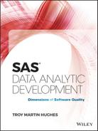
For example, when the SORT procedure runs with multithreading enabled, SAS divides the initial data set into numerous smaller data sets, sorts these in parallel, and finally joins the sorted subsets into a composite, sorted data set. Figure 9.1 depicts the modest performance improvement that the SORT procedure achieves through multithreading on two CPUs. On systems that were tested, increasing CPUCOUNT beyond two CPUs failed to increase performance further.
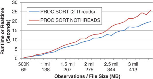
Figure 9.1 Multithreaded versus Single-Threaded SORT Procedure
Multithreading facilitates the optimization of threads by the SAS application by evenly distributing threads across processors. Moreover, because only one instance of the SAS application is running, system resource overhead is minimized. Notwithstanding, SAS practitioners can improve performance of the SORT procedure by running multiple procedures in parallel. For example, the following code simulates parallel processing of the SORT procedure for the PERM.Mydata data set, which has 1,000 observations:
* first sort module to run in parallel;
proc sort data=perm.mydata (firstobs=1 obs=500) out=sort1;
   by num1;
run;
* second sort module to run in parallel;
proc sort data=perm.mydata (firstobs=501 obs=1000) out=sort2;
   by num1;
run;
data sorted;
   set sort1 sort2;
   by num1;
run;
An initial process (not shown) would determine how many parallel processes to run (based on file size or observation count), after which two (or more) SAS sessions could be spawned with the SYSTASK statement to perform the sorting. After the batch jobs had completed, a final DATA step in the original SAS program would rejoin the two sorted halves for a faster solution than the native SORT procedure.
Two primary methods exist for implementating parallel processing in SAS software. The first, as described previously, uses an engine (AKA controller or driver) to spawn multiple SAS sessions to execute external code in parallel. For example, the values for FIRSTOBS, OBS, and the output data set name for each SORT procedure would be dynamically encoded so that external code (not shown) could be called with SYSTASK and executed. The second method (demonstrated in the following section) uses software that is actually designed to have two or more instances run simultaneously so that they can work together to accomplish some shared task (like sorting) faster.
Distributed SORT-SORT-MERGE
The SORT-SORT-MERGE represents the common task of joining two data sets by some unique key or keys. The process can be accomplished using the SQL procedure or hash object but is often performed by two successive SORT procedures followed by a DATA step that joins the two data sets:
proc sort data=temp1;
   by num1;
run;
proc sort data=temp2;
   by num1;
run;
data sorted;
   merge temp1 temp2;
   by num1;
run;
This code creates a false dependency, described in the “False Dependencies of Process” section in chapter 7, “Execution Efficiency,” because the sorts are not dependent on each other yet are performed in series rather than parallel. Especially where the two data sets are equivalent in size and take roughly the same amount of time to sort, the speed of the SORT-SORT-MERGE can be increased by performing the two sorts in parallel. To coordinate this, SAS software should be written that is dynamically capable of sorting either Temp1 or Temp2 based on whichever data set has not been sorted. Thus, when two instances of the software are executed simultaneously, one will sort Temp1 and the other—detecting that Temp1 has already commenced its sort—will sort Temp2. When both SORT procedures complete, one of the software instances will perform the merge while the other patiently waits or exits. A similar technique is demonstrated in the “Executing Software in Parallel” section in chapter 7, “Execution Efficiency,” to perform independent MEANS and FREQ procedures in parallel.
The following code initializes the PERM.Data1 and PERM.Data2 data sets—each of which contains 100 million observations—that will be individually sorted and subsequently merged:
libname perm 'C:perm';
data perm.data1 (drop=i);
   length num1 8 char1 $10;
   do i=1 to 100000000;
      num1=round(rand('uniform')*1000);
      char1='data1';
      output;
      end;
run;
data perm.data2 (drop=i);
   length num1 8 char2 $10;
   do i=1 to 100000000;
      num1=round(rand('uniform')*1000);
      char2='data2';
      output;
      end;
run;
The following code should be saved as C:permdistributed.sas. The program can be run in series in a single SAS session, which will perform the typical SORT-SORT-MERGE in succession. For faster performance, however, the software can be opened in two different SAS sessions and run simultaneously. The two SORT procedures will perform in parallel, after which one of the sessions will merge the two data sets into the composite PERM.Merged:
libname perm 'C:perm';
%include 'C:permlockitdown.sas';
%macro control_create();
%if %length(&sysparm)>0 %then %do;
   data _null_;
      call sleep(&sysparm,1);
   run;
   %end;
%if %sysfunc(exist(perm.control))=0 %then %do;
   %put CONTROL_CREATE;
   data perm.control;
      length process $20 start 8 stop 8 jobid 8;
      format process $20. start datetime17. stop datetime17. jobid 8.;
   run;
   %end;
%mend;
%macro control_update(process=, start=, stop=);
data perm.control;
   set perm.control end=eof;
%if %length(&stop)=0 %then %do;
   output;
   if eof then do;
   process="&process";
   start=&start;
   stop=.;
   jobid=&SYSJOBID;
   output;
   end;
   %end;
%else %do;
   if process="&process" and start=&start then stop=&stop;
   %end;
   if missing(process) then delete;
   run;
&lockclr;
%mend;
%macro sort(dsn=);
%let start=%sysfunc(datetime());
%control_update(process=SORT &dsn, start=&start);
proc sort data=&dsn;
   by num1;
run;
%lockitdown(lockfile=perm.control, sec=1, max=5, type=W, canbemissing=N);
%control_update(process=SORT &dsn, start=&start, stop=%sysfunc(datetime()));
%mend;
%macro merge();
%let start=%sysfunc(datetime());
%control_update(process=MERGE, start=&start);
data perm.merged;
   merge perm.data1 perm.data2;
   by num1;
run;
%lockitdown(lockfile=perm.control, sec=1, max=5, type=W, canbemissing=N);
%control_update(process=MERGE, start=&start, stop=%sysfunc(datetime()));
%mend;
%macro engine();
%let sort1=;
%let sort2=;
%let merge=;
%control_create();
%do %until(&sort1=COMPLETE and &sort2=COMPLETE and &merge=COMPLETE);
   %lockitdown(lockfile=perm.control, sec=1, max=5, type=W,    canbemissing=N);
   data control_temp;
      set perm.control;
      if process='SORT PERM.DATA1' and not missing(start) then do;
         if missing(stop) then call symput('sort1','IN PROGRESS'),
         else call symput('sort1','COMPLETE'),
         end;
      else if process='SORT PERM.DATA2' and not missing(start) then do;
         if missing(stop) then call symput('sort2','IN PROGRESS'),
         else call symput('sort2','COMPLETE'),
         end;
      else if process='MERGE' and not missing(start) then do;
         if missing(stop) then call symput('merge','IN PROGRESS'),
         else call symput('merge','COMPLETE'),
         end;
   run;
   %if %length(&sort1)=0 %then %sort(dsn=PERM.DATA1);
   %else %if %length(&sort2)=0 %then %sort(dsn=PERM.DATA2);
   %else %if &sort1=COMPLETE and &sort2=COMPLETE and %length(&merge)=0     %then %merge;
   %else %if &sort1ˆ=COMPLETE or &sort2ˆ=COMPLETE or    &mergeˆ=COMPLETE %then %do;
      &lockclr;
      data _null_;
         call sleep(5,1);
         put 'Waiting 5 seconds';
      run;
      %end;
   %else &lockclr;
   %end;
%mend;
%engine;
The control table (PERM.Control) depicted in Table 9.1 demonstrates the performance improvement: each data set was sorted in approximately four minutes in parallel, after which the %MERGE macro merged the two data sets. Note that the JOBID variable indicates that two separate jobs were running.
Table 9.1 Control Table Demonstrating Parallel Processing
| Process | Start | Stop | JobID |
| SORT PERM.DATA1 | 01APR16:13:16:23 | 01APR16:13:20:15 | 14776 |
| SORT PERM.DATA2 | 01APR16:13:16:26 | 01APR16:13:21:01 | 13368 |
| MERGE | 01APR16:13:21:01 | 01APR16:13:21:56 | 13368 |
Another example of distributed processing is found in the “Executing Software in Parallel” section in chapter 7, “Execution Efficiency.” Whether the SYSTASK statement is used to spawn separate SAS sessions or a control table is used to broker and coordinate separate SAS sessions that are operating concurrently, parallel processing can provide significantly faster processing.
LOAD SCALABILITY
Load scalability describes the ability of a system or software to accommodate data throughput of increasing volume or velocity. Variability—the third V in the big data triad—represents less of a scalability challenge and more of a robustness challenge when unexpected or invalid data are encountered that are not handled through appropriate quality controls. Load scalability is arguably the most relevant scalability facet to data analytic development because of the inherent accretionary nature of data sets, databases, data streams, and other data sources. In fact, scaling resources (by increasing hardware) and scaling demand (by increasing the instances of SAS software executing in parallel) are often necessitated to enable SAS software to scale successfully as load increases.
The expectations of software scalability vary intensely with software intent. User-focused applications typically demand instantaneous service without delay, regardless of data volume. For example, a Google search today should be just as quick and effective as a Google search in a year when the quantity of searchable data may have doubled. In the applications world, scalability generally denotes no change in performance as data volume scales. And, in recent years, SAS has promulgated several in-memory solutions, such as SAS In-Memory Statistics and SAS Visual Analytics, which provide instantaneous processing, scaling effectively without diminished performance.
Base SAS, however, traditionally supports data analytic endeavors rather than applications development. In data analytic environments, users are typically not waiting for an instantaneous response as is common in software and web applications. Thus, in many SAS environments, as data load increases, execution time is not only allowed to but also expected to commensurately increase. For example, if a data set doubles in size within a year, for many purposes it's acceptable that the time to sort those data equivalently doubles, or at least follows a predictable algorithm. In data analytic environments, a scalable solution is more commonly defined as one that continues to operate efficiently despite greater throughput while software applications more commonly define scalability as equivalent performance, especially software execution time.
This disparity is demonstrated in Figure 9.2, which contrasts the scalability required by user-focused applications such as a Google search with the scalability demonstrated by a process in data analytic software.
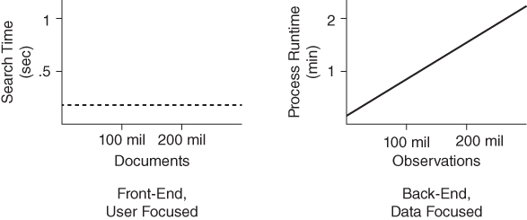
Figure 9.2 Contrasting Scalability Performance
For example, in data analytic development, as long as the correlation of file size and execution time for the SORT procedure remains linear, scalability is demonstrated and the efficiency of the procedure remains stable. Thus, while increased resources are often utilized as the software scales to respond to larger data sets, the resources are consumed at the same rate. Efficiency can begin to decrease as increasingly more resources are utilized, however, and as system resources (such as CPU cycles or memory) are depleted, a threshold may be reached after which the process performs inefficiently and thereafter fails. This type of failure is described later in the “Inefficiency Elbow” section.
In other cases, however, data analytic processes may have fixed performance thresholds that cannot be surpassed. For example, an hourly financial fraud program may be required by organizational policy to run every hour; despite increasing data volume (or velocity), this threshold represents a steadfast performance requirement. Given these requirements, and likely having exhausted programmatic methods to improve software speed, stakeholders would need to achieve scalability through nonprogrammatic methods that either scale resources or scale demand. In all cases, a shared understanding of load scalability by all stakeholders must be achieved given the variability in defining what constitutes and does not constitute scalable performance.
Data Volume
Data volume describes the size of a data set or data product, commonly measured and referenced as file size or observation count. The number of observations can be useful in tracking incremental data sources as well as validating processes in which the number of observations is expected to increase, decrease, or remain constant. Observation count is often anecdotally used in SAS literature to describe or make claims to “big data,” although this is a poor metric when used in isolation. Blustering about a “10 billion-observation data set”—without additional context—conveys little more than hype. In most circumstances, file size represents a more useful, quantifiable, comparable metric for conveying the enormity of data.
Big data became a focus of the data analytic community because scalability challenges were encountered and overcome, but the challenges almost exclusively arise from file size—not observation count. File size is critical to understanding data volume because it influences the performance of input/output (I/O)-bound processes such as reading or writing data. The %HOWBIG macro in the “Data Governors” section depicts a reusable macro that programmatically assesses file size and which can be used in calculating actual and predicted data volume to avoid and overcome scalability challenges.
Diminished Performance
As demonstrated in Figures 9.1 and 9.2, when data volume increases, performance generally will slow as additional system resources are consumed to handle the additional load. Performance typically decreases in a predictable, often linear path correlated most significantly with file size. This increased execution time can cause software to fall short of performance requirements. For example, if an ETL process is required by a customer to complete in 55 minutes, as data volume increases over the software lifespan, execution time may increase until it fails to meet this performance objective.
In many cases, performance requirements are predicated upon temporal or other limitations. For example, the requirement that software execute in less than 55 minutes may exist because the ETL program is intended to be run every hour. Thus, failure to complete in a timely manner might cause dependent processes to fail or might delay or hamper the start of the subsequent hourly execution. In a robust, fault-tolerant system, while runtime errors will not be produced by these failures, business value can be diminished or eliminated when dependent processes cannot execute. This phenomenon is discussed more in the “Functional Failures” section.
As data volume increases, or when it's expected to increase in the future, it's important for developers and other stakeholders to understand customer intent regarding software execution time limits. For example, requiring that software must complete in 55 minutes or less is very different from requiring that software must produce output every 55 minutes. In the first example, the customer clearly specifies that from the moment data are received, they should be extracted, transformed, and loaded and ready for use in 55 minutes. However, if the customer only wants data updated once per hour, it may be acceptable to create a program flow that takes 90 minutes, but that is run in parallel and staggered to still achieve output once per hour.
Figure 9.3 demonstrates two interpretations of the 55-minute requirement. On the left, the phase-gate approach is shown across a four-hour time period, demonstrating the requirement that the software complete in 55 minutes or less without the ability to overlap any processes. On the right, an overlapping schedule is demonstrated in which two copies of the software are able to run for 90 minutes, but because one starts on even hours and one starts on odd hours, they collectively produce results once an hour. In this example, the extract module is able to overlap with the load module to facilitate parallel processing and a control table or other mechanism would be required to coordinate the concurrent activities.

Figure 9.3 Phase-Gate and Parallel Software Models
Parallel execution and other distributed processing models are a primary method to reduce execution time of software as data volume increases. Another benefit of the overlapping execution method noted in Figure 9.3 is the tendency to process smaller data sets, which reduces execution time. For example, an ordinary serialized ETL process that completed in 90 minutes would only ingest incoming data every 90 minutes. However, because the parallel version ingests data every 60 minutes, smaller chunks are being processed each time, thus reducing overall execution time.
Inefficiency Elbow
The inefficiency elbow represents a specific type of performance failure that occurs as resources are depleted due to increased data volume. Because execution time is the most commonly assessed performance metric, the elbow is typically first noticed when software performance drastically slows due to a relatively nominal increase in data volume. Figure 9.4 demonstrates the inefficiency elbow within the SAS University Edition, observed when execution times for the SORT procedure are measured in 100,000 observation increments from 100,000 to 4.5 million observations. Execution time takes only 36 seconds at 4.2 million observations, 98 seconds at 4.3 million observations, and 4 hours 21 minutes by 4.5 million observations!

Figure 9.4 Inefficiency Elbow on SORT Procedure
The inefficiency elbow depicts the relative efficiency of a process as it scales to increasing data volume, indicating relatively efficient performance to the left of the elbow and relatively inefficient performance to the right. This is to say that efficient performance does not necessarily denote that the code in the underlying process is coded as efficiently as possible, only that as data volume scales, the software less efficiently utilizes resources until it fails outright.
To better understand what occurs as the efficiency elbow is reached, Table 9.2 demonstrates abridged UNIX FULLSTIMER performance metrics, including real time, CPU time, memory, OS memory, switch counts, page faults, involuntary context switches, and block input operations. SAS documentation contains more information about these specific metrics.3 Metrics surrounding the inefficiency elbow (from 3.5 to 4.5 million observations) demonstrate the substantial increase in I/O processing as SAS shifts from RAM to virtual memory, and finally the later jump in CPU usage.
Table 9.2 FULLSTIMER Metrics for SORT Procedure at Inefficiency Elbow
| OBS | File Size (MB) | Seconds | User CPU Time | System CPU Time | Memory | OS Memory | Switch Count | Page Faults | Invol Switches | Block In Ops |
| 3,500,000 | 482 | 29 | 17.96 | 5.59 | 675.36 | 706.1 | 41 | 0 | 666 | 0 |
| 3,600,000 | 496 | 30 | 18.68 | 5.86 | 694.56 | 725.3 | 41 | 0 | 602 | 0 |
| 3,700,000 | 509 | 31 | 19.27 | 5.76 | 713.76 | 744.51 | 49 | 1 | 712 | 32 |
| 3,800,000 | 523 | 33 | 19.37 | 6.34 | 732.96 | 763.71 | 49 | 9 | 553 | 352 |
| 3,900,000 | 537 | 39 | 20.11 | 6.98 | 747.37 | 778.11 | 49 | 200 | 717 | 6552 |
| 4,000,000 | 551 | 35 | 20.29 | 7.96 | 766.57 | 797.32 | 49 | 47 | 987 | 2640 |
| 4,100,000 | 564 | 36 | 21.4 | 7.41 | 785.77 | 816.52 | 49 | 39 | 962 | 2128 |
| 4,200,000 | 578 | 98 | 20.36 | 14.87 | 806.54 | 837.29 | 97 | 5663 | 2546 | 338608 |
| 4,300,000 | 592 | 190 | 13.03 | 31.83 | 825.74 | 856.49 | 249 | 35156 | 3744 | 1213088 |
| 4,400,000 | 606 | 264 | 9.91 | 20.46 | 844.94 | 875.69 | 185 | 21417 | 3077 | 836704 |
| 4,500,000 | 620 | 15679 | 0.02 | 521.79 | 864.14 | 894.89 | 1083 | 893270 | 15978 | 34001456 |
As Figure 9.2 demonstrates, although the inefficiency elbow is not reached until around 4.2 million observations (as defined by the change in execution time), I/O metrics presaged defeat of the SORT procedure several iterations earlier. For example, both page faults and block input operations had consistently been 0 until 3.7 million observations, when both began increasing. Given this information, a quality assurance process monitoring these metrics could have detected levels above some threshold and subsequently terminated the process. This technique is described in the following section, “Data Governors.”
Without understanding the contributing factor that increased data volume can play in inefficiency, stakeholders may mistakenly attribute process slowness to network or other infrastructure issues. Worse yet, stakeholders may accept reduced performance as the status quo and their penance for big data, rather than investigating the cause of performance deficiencies. In reality, several courses of action can either move or remove the inefficiency elbow, the first of which begins with stress testing to determine what volume of data will induce inefficiency or failure in specific DATA steps, SAS procedures, and other processes. Without proper stress testing, discussed in the “Stress Testing” section in chapter 16, “Testability,” the inefficiency elbow will be a very unwelcome surprise when it's encountered.
To reduce the effects of the inefficiency elbow, stakeholders have several programmatic and nonprogrammatic solutions that entail more efficient use of resources, more distributed use of resources, or procurement of additional system resources:
- More efficient software—The inefficiency elbow denotes a change in relative efficiency; thus, it's possible that software is not truly operating efficiently even to the left of the elbow. For example, in Figure 9.4, it's possible that a WHERE statement in the SORT procedure—if appropriate—would reduce the number of observations read, thus reducing I/O consumption and shifting the elbow to the right.
- Increased infrastructure—Increased infrastructure can include increasing the hardware components as well as installing distributed SAS solutions such as SAS Grid Manager or third-party solutions like Teradata or Hadoop. By either increasing system resources or increasing the efficiency with which those resources can be utilized, the inefficiency elbow is shifted to the right, allowing more voluminous data to be processed with efficiency.
- Distributed software—As demonstrated in Figure 9.3, when processes can overlap or be run in parallel, the resource burden exhibited by a single SAS session can be distributed across multiple sessions and processors. Moreover, when this parallel design distributes data volume across multiple sessions, this doesn't alter the inefficiency elbow, but does decrease the position of execution time on the graph since fewer observations are processed through each independent SAS session.
- Data governors—A data governor is a quality control device that restricts data injects based on some criteria such as file size. For example, if a certain process is stress tested and demonstrates relative inefficiency when processing data sets larger than 1 GB, a data governor placed at 1 GB would block or subset files (for later or parallel processing) to prevent inefficiency.
Figure 9.5 demonstrates the effect of these methods on software performance and the inefficiency elbow.

Figure 9.5 Inefficiency Elbow Solutions
SAS literature is replete with examples of how to design SAS software that is faster and more efficient, so these best practices are not discussed in this text. Infrastructure is discussed briefly in the “Distributed SAS Solutions” section, but this also lies outside of the focus of this text. Parallel processing and distributed solutions are discussed throughout chapter 7, “Execution Efficiency,” and data governors are discussed in the following section.
Data Governors
Just as a governor in a vehicle is installed to limit speed beyond some established threshold, a data governor can limit the velocity or, more typically, the volume of data for specific processes. Data governors can be implemented immediately before the inefficiency elbow, as demonstrated in Figure 9.5, or anywhere else to ensure a process does not begin to function inefficiently or fail. While data volume is the primary factor affecting performance, other factors can also lead to more substantial variability. For example, if other memory-hogging processes are already running, performance or functional failure might be reached at a significantly lower data volume because resources are more constrained. The “Contrasting the SAS University Edition” section in chapter 10, “Portability,” also demonstrates the influence that nonprogrammatic factors such as SAS interface have on the inefficiency elbow.
A data governor must first determine the file size of the data set. The following %HOWBIG macro obtains the file size in megabytes from the DICTIONARY.Tables data set. Note that a generic return code—the global macro variable &HOWBIGRC—is generated to facilitate future exception handling. However, robust production software would need to implement additional controls—for example, to validate that a data set exists and is not exclusively locked by another process, either of which would cause the SQL procedure to fail:
%macro howbig(lib=, dsn=);
%let syscc=0;
%global howbigRC;
%global filesize;
%global nobs;
%let howbigRC=GENERAL FAILURE;
proc sql noprint;
   select filesize format=15.
      into :filesize
      from dictionary.tables
      where libname=%upcase("&LIB") and memname=%upcase("&DSN");
   select nobs format=15.
      into :nobs
      from dictionary.tables
      where libname=%upcase("&LIB") and memname=%upcase("&DSN");
   quit;
run;
%if %eval(&syscc>0) %then %do;
   %let howbigRC=&syscc;
   %let filesize=;
   %let nobs=;
   %end;
%else %do;
   %let filesize=%sysevalf(&filesize/1048576); *convert bytes to MB;
   %let nobs=%sysevalf(&nobs);
   %end;
%if &syscc=0 %then %let howbigRC=;
%put filesize: &filesize;
%put observations: &nobs;
%mend;
In this example, the inefficiency elbow was shown to be around 1GB, so to account for some variability, the data governor will be set at 0.9 GB through conditional logic similar to the following code:
%let governor=%sysevalf(1024*.9); * in MB;
%if %sysevalf(&filesize>&governor) %then %do;
   * subset the data here or perform other busines logic;
   %end;
* run process on full data set or data subset;
If a 1.25 GB data set is encountered by the governor, business logic could specify that the first 0.9 GB of the data set be processed initially and the last 0.35 GB be processed either in series—that is, after the first batch completes—or immediately as a parallel process. One facile way to implement a data governor is through FIRSTOBS and OBS statements that can be used to subset the data before it is even read, efficiently eliminating unnecessary I/O processing. Because FIRSTOBS and OBS are dependent on observation number while data governors and other performance quality controls should be driven by file size, a conversion to observation count is necessary.
In a separate example, the following code demonstrates the creation of the 1 million-observation PERM.Mydata data set which, when interrogated through the %HOWBIG macro, is shown to be 7.875 MB:
libname perm 'c:perm';
data perm.mydata (drop=i);
   length num1 8;
   do i=1 to 1000000;
      num1=round(rand('uniform')*10);
      output;
      end;
run;
Suppose that stress testing has indicated that efficiency begins to decrease shortly after 6 MB (apparently this process has time-traveled back to 1984), indicating that the governor should be installed at 6 MB. The following macro %SETGOVERNOR calls the %HOWBIG macro to determine the file size and observation count and, if the file size exceeds the 6 MB limit, then the value to be used in the OBS option (to ensure a file size equal to or less than 6 MB) will be initialized in the &GOV macro variable.
* determines file size and provides the observation number for OBS;
%macro setgovernor(lib=, dsn=, govMB=);
%let syscc=0;
%global setgovernorRC;
%global governor;
%local gov;
%let setgovernorRC=GENERAL FAILURE;
%let governor=;
%howbig(lib=&lib, dsn=&dsn);
%if %length(&howbigRC)>0 %then %do;
   %let setgovernorRC=HOWBIG failure: &howbigRC;
   %return;
   %end;
%if %sysevalf(&filesize>&govMB) %then %do;
   %let gov=%sysfunc(round(%sysevalf(&nobs * &govMB / &filesize)));
   %let governor=(firstobs=1 obs=&gov);
   %end;
%if &syscc=0 %then %let setgovernorRC=;
%mend;
The following code invokes the %SETGOVERNOR macro to determine how many observations should be read into the Test data set. Because the file size 7.875 MB is greater than the 6 MB governor, the OBS statement (codified in the &GOVERNOR macro variable) specifies that only 761,905 observations (or 1,000,000 × 6 / 7.875) should be read into the Test data set.
%setgovernor(lib=perm, dsn=mydata, govMB=6);
data test;
   set perm.mydata &governor;
run;
To test the accuracy of this math, the %HOWBIG macro can subsequently be run on the Test data set, which produces the following output, indicating that the data set is indeed now only 6 MB and equal to the established governor.
%howbig(lib=work, dsn=test);
NOTE: PROCEDURE SQL used (Total process time):
      real time           0.00 seconds
      cpu time            0.00 seconds
filesize: 6
observations: 761905
In this example, accuracy of the subset data set size is guaranteed because the data set was created through a standardized process, thus all observations are of equal size. In more variable data sets or especially in heteroscedastic data sets in which the file size of each observation is correlated with the observation number itself (e.g., values are more likely to be blank in the first half of the data set than the second half), this method will be less accurate. In many situations, however, this type of data governance provides an effective means to limit input into some process so that it does not incur performance or functional failures due to high data volume. And, depending on business logic, the remaining observations that were excluded could be executed in parallel or in series following the completion of the first process.
Data governors are most effective when inter-observation comparisons are not required. For example, if the DATA step had included by-level processing, utilized the RETAIN or LAG functions, or otherwise required interaction between observations, the data set could not have been split so easily. In some instances, it's possible to take the last observation from the first file and replicate this in the second file, thus providing continuity between the data set chunks. In other cases, such as a data governor placed on the FREQ procedure, the output from each respective FREQ procedure would need to be saved via the OUT statement and subsequently combined to produce a composite frequency table. Notwithstanding these complexities, where resources are limited and inefficiency overshadows big data processing, data governors can be a cost-effective, programmatic solution to scaling to big data.
As discussed, the %HOWBIG macro does not detect specific exceptions that could occur, such as a missing or exclusively locked data set that would cause the SQL procedure to fail. However, it includes basic exception handling to detect general failures via the &SYSCC global macro variable. The return code &HOWBIGRC is initialized to GENERAL FAILURE and is only set to a missing value (i.e., no failure present) if no warnings or runtime errors are detected. The %SETGOVERNOR macro follows an identical paradigm but, because it calls %HOWBIG as a child process, %SETGOVERNOR must dynamically handle failures that may have occurred in %HOWBIG through exception inheritance. Inheritance is required to achieve robustness in modular software design and is introduced in the “Exception Inheritance” section in chapter 6, “Robustness.”
Functional Failures
As data volume continues to increase and as system resources continue to be depleted, functional failure can become more likely; SAS software can terminate with a runtime error because it runs out of CPU cycles or memory. In some instances, the inefficiency elbow will have first been reached, indicating that performance will have slowed substantially as the process became less efficient. In other cases, the inefficiency elbow may not exist but a performance failure will occur because the execution time exceeds thresholds established in requirements documentation. Still, in other cases, some processes fail with runtime errors with no prior performance indicators (aside from FULLSTIMER metrics that may not have been monitored).
Figure 9.6 demonstrates performance of the SORT procedure when the volume of data is varied from 100,000 to 5 million observations. In a development environment that espouses software development life cycle (SDLC) principles, load testing would have demonstrated performance of the procedure at the predicted load of 2 million observations. However, realizing that data volume might increase over time, additional stress testing would have tested increasingly higher volumes of data to determine where performance and functional failures begin to occur.
Figure 9.6 Scaling with Efficiency
If an inefficiency elbow is demonstrated through stress testing, performance requirements for execution time and resource consumption should be established below that point. To ensure that this threshold is never crossed, a data governor can be implemented to prevent both performance failures and functional failures from occurring when exceptionally large data sets are encountered. Figure 9.6 demonstrates the placement of these elements to support efficient performance.
Even with adequate technical requirements, robust quality control measures such as data governors, and attentive monitoring of system resources, SAS processes can still fail due to resource consumption while processing big data. For this reason, production software should espouse fault-tolerant programming within an exception handling framework that monitors all completed processes for warnings and runtime errors that can signal functional failures due to resource constraints. The use of return codes and global macro variable error codes such as &SYSCC and &SYSERR that facilitate failing safe are discussed extensively in chapter 3, “Communication,” and chapter 6, “Robustness.”
Data Velocity
Data velocity typically describes the rate at which data are processed or accumulate. In this usage, when velocity increases, it will often also increase data volume. For this reason, the challenges of increased data velocity will only be discussed briefly in this section. But velocity can also describe a change in requirements in which data are required to be processed faster. Both data-driven and requirements-driven velocity increases can cause performance and functional failures.
Data-driven velocity increases result from data pouring into a system at a faster rate. Because data are often processed in batches at set intervals, such as every 15 minutes, this increased velocity can cause these chunks to grow in size, at which point they also represent increased data volume. As demonstrated in the prior “Data Volume” section, data volume can pose serious challenges to SAS processes. The second failure pattern occurs not when the actual pace of data increases but when the requirements for some process are increased. For example, an ETL process initially was mandated to run hourly and a customer has now required that it be run every 15 minutes. While this will mean fewer data must be processed at every 15-minute interval, the processing must now occur in one-fourth the time. While the cause is requirements-driven, the challenge simulates other scalability issues in which too many data exist to be processed within some time-boxed period.
Velocity as an Indicator
During planning and design, at least a rough conception of eventual data volume should be obtainable. In many data analytic development environments, the data are already held so velocity is zero. For example, clinical trials software might be developed to analyze a study sample that has already been collected and to which data are not being added. In other cases, however, data accumulate at some velocity, which can be useful in predicting future data volume. For example, clinical trials software might be developed to analyze a longitudinal study that is expected to continue to grow in size for five years. Knowledge of data velocity can be used to establish load testing parameters to determine if performance requirements will be adequate throughout the life of the software. If an initial data set has 10,000 observations and is expected to grow by 10,000 observations each year thereafter, performance requirements would need to expect file sizes of 50,000 to 60,000 observations.
Modest file sizes such as this likely would not incur any noticeable performance decreases, so neither data volume nor velocity would be of significant concern in this example. But in environments where data volume can be staggering, data velocity should be used to facilitate accurate load and stress testing at accurate data volume levels. This information can be critical to stakeholders, helping them predict when software or hardware upgrades will be needed to maintain equivalent performance.
To continue the example demonstrated in Figure 9.6, the current data volume of some SAS processes is 2 million observations. If stakeholders further determine that the volume will grow by approximately 1 million observations per year, then they can predict that the process will still be operating efficiently and within the stated performance requirement of two hours' execution time. However, if data velocity instead accelerates, performance or functional failures could result as data volume increases and the software takes longer and longer to run. This underscores the importance of establishing expected software lifespan during planning and design phases of the SDLC.
The ability to predict future software performance is beneficial to Agile software development environments in which stakeholders aim to release software incrementally through rapid development that delivers small chunks of business value. An initial SAS process that meets performance requirements could be developed quickly and released, with the understanding that subsequent incremental releases will improve this performance to ensure that performance requirements will be met in the future as data volume continues to increase. Progressive software requirements to facilitate increasing the performance of software over time are discussed in the “Progressive Execution Time” section in chapter 7, “Execution Efficiency.”
The role of data volume and velocity in supporting effective Agile development is demonstrated in Figure 9.7. In this example, an initial solution is released in the first iteration that meets the two-hour performance requirement but that would begin to fail to meet this requirement when the data volume increased to approximately 2.5 million observations. The software is refactored in the second iteration to produce faster performance, which shifts the predicted performance function (as estimated through load and stress testing). After refactoring a second time in the third iteration, the software performance increases to a level that will meet the performance requirements to 5 million observations, giving stakeholders ample time to decide how to handle that scalability challenge when it is encountered. Thus, Agile development enables SAS practitioners to produce a solution quickly that meets immediate requirements while allowing developers to keep an eye toward the future and eventual performance requirements that software will need to meet to scale to larger data. This forward-facing awareness is the objective of software refactoring and extensibility, discussed in the “From Reusability to Extensibility” sections in chapter 18, “Extensibility.”

Figure 9.7 Incremental Refactoring to Support Increased Software Performance
Scalability Idiosyncrasies
Load scalability is typically construed as causing performance failures (due to increased execution time) or functional failures (due to depleted system resources). However, increased data volume can also indirectly cause idiosyncratic results, runtime errors, and other failures. This further underscores the necessity of stress testing all production software to determine where syntax might need to be made more flexible to adapt to shifts in business logic or Base SAS system thresholds. These two issues are discussed in the following sections.
Invalid Business Logic
Invalid business logic essentially amounts to errors that SAS practitioners make in software design when they fail to predict implications of higher data volume. The failure patterns are endless but one example occurs when observation counters exceed predicted limits. For example, the following code simulates an ingestion process (with increasing data volume) followed by a later process:
libname perm 'c:perm';
* simulates data ingestion;
data perm.mydata;
   length num1 8;
   do i=1 to 1000;
      num1=round(rand('uniform')*10);
      output;
      end;
run;
* simulates later data process;
filename outfile 'c:permmydata_output.txt';
data write;
   set perm.mydata;
   file outfile;
   put @1 i @4 num1;
run;
The output demonstrates that the second process will operate effectively when the data set contains fewer than 100 observations, but when this threshold is crossed, the data no longer are delimited by a space and are indistinguishable. At 1,000 observations, a functional failure occurs when the data are overwritten:
1  4
2  1
3  4
...
9  1
10 7
11 6
...
99 0
1008
1013
Logic errors such as this are easily remedied but can be difficult to detect. However, if load testing and stress testing are not performed or fail to detect underlying software defects, they can go unnoticed indefinitely.
SAS Application Thresholds
Programmatic limitations exist within the SAS Base language just as in any software language. For example, variable naming conventions specify acceptable alphanumeric characters that can appear in a SAS variable name, and maximum name lengths are specified for SAS variables, macro variables, libraries, and other elements. Under the SAS 9.4 variable naming standard (V7), both data set variable names and macro variable names are limited to 32 characters in length. Thus, failures could result if variable names were being dynamically created through macro language, if the name included an incrementing number, and if that number caused the length of the variable to exceed 32 characters. Many of these SAS thresholds are detailed in SAS® 9.4 Language Reference: Concepts: Fifth Edition.4
Other SAS language limitations, however, are published nowhere and are discovered solely through trial and error—that is, when software has been performing admirably, but suddenly and inexplicably fails. For example, a commonly cited method to determine the number of observations in a data set is to utilize the COUNT statement in the SQL procedure to create a macro variable. The following output demonstrates that the PERM.Mydata data set has 1,000 observations:
proc sql noprint;
   select count(*)
   into :nobs
   from perm.mydata;
quit;
%put OBS: &nobs;
OBS: 1000
While this method lacks robustness (because the SQL procedure fails with a runtime error if the data set does not exist, is exclusively locked, or contains no variables), it can be a valuable tool when these exceptions are detected and controlled through exception handling. But as data volume increases, another exception can occur when the default SAS variable format shifts from standard to scientific notation. Thus, 10 million is represented in standard notation as 10000000, while 100 million is represented in scientific notation as 1E8:
%put OBS: &nobs; * for 10 million observations;
OBS: 10000000
%put OBS: &nobs; * for 100 million observations;
OBS: 1E8
This notational shift can destroy SAS conditional logic and other processes, creating aberrant results. For example, if %SYSEVALF is not used to compare the resultant value, then operational comparisons are character—not numeric—which causes scientific notation to yield incorrect results:
* equivalent values in standard and scientific notation;
%let nobs_stand=100000000;
%let nobs_sci=1E8;
%macro test(val=);
%if &nobs_stand<9 %then %put standard notation: 100000000 is less than &val;
%else %put standard notation: 100000000 is NOT less than &val;
%if &nobs_sci<9 %then %put scientific notation: 1E8 is less &val;
%else %put scientific notation: 1E8 is NOT less than &val;
%mend;
%test(val=9);
standard notation: 100000000 is NOT less than 9
scientific notation: 1E8 is less 9
1E8 is not less than 9, but when a character comparison is made, the fallacy is demonstrated because SAS only assesses that the first character, 1, is less than 9. The %EVAL function is used to force numeric comparisons in the macro language and typically works—that is, until scientific notation is encountered:
%macro test(val=);
%if %eval(&nobs_stand<9) %then %put standard notation: 100000000 is less than &val;
%else %put standard notation: 100000000 is NOT less than &val;
%if %eval(&nobs_sci<9) %then %put scientific notation: 1E8 is less &val;
%else %put scientific notation: 1E8 is NOT less than &val;
%mend;
%test(val=9);
standard notation: 100000000 is NOT less than 9
scientific notation: 1E8 is less 9
The scientific notation unfortunately fails again, but now for a different reason. The %EVAL function does not recognize scientific notation and thus views this as an attempt to convert a character value to a number. This is demonstrated in the following output that results when the %EVAL function is used to print standard and scientific notation:
%put standard: %eval(&nobs_stand);
standard: 100000000
%put scientific: %eval(&nobs_sci);
ERROR: A character operand was found in the %EVAL function or %IF condition where a numeric operand is required. The condition was: 1E8
scientific:
This failure is overcome by substituting the %EVAL function with the %SYSEVALF function, which does interpret scientific notation. Now, as expected, both standard and scientific notation are accurately read and can be operationally evaluated:
%macro test(val=);
%if %sysevalf(&nobs_stand<9) %then %put standard notation: 100000000 is less than &val;
%else %put standard notation: 100000000 is NOT less than &val;
%if %sysevalf(&nobs_sci<9) %then %put scientific notation: 1E8 is less &val;
%else %put scientific notation: 1E8 is NOT less than &val;
%mend;
%test(val=9);
standard notation: 100000000 is NOT less than 9
scientific notation: 1E8 is NOT less than 9
While %SYSEVALF is not always required and can be replaced by %EVAL for many operations, as data sets increase in volume, %SYSEVALF may be required to ensure that scientific notation is accurately assessed. Another possible solution is to add FORMAT=15. to the SELECT statement in the SQL procedure, as demonstrated previously in the “Data Governors” section. The duality of these two solutions is discussed further in the “Risk versus Failure” section in chapter 1, “Introduction.”
SCALABILITY IN THE SDLC
The role that scalability plays throughout the SDLC is emphasized in the “Load Scalability” section, demonstrating that scalability should be something you plan for in software, not something that happens to software unexpectedly. Through load testing and stress testing, SAS practitioners should be able to demonstrate with relative certainty the performance and efficiency that software will exhibit as it scales. With robust design that avoids inefficiency through data governors and other controls, and fault-tolerant design that detects and responds to runtime errors experienced when software fails to scale, software reliability should not be diminished as it encounters big data.
One of the most important reasons to understand predicted load scalability as early as possible in the SDLC is that it can alert stakeholders to future actions that they may need to take to ensure software performance objectives continue to be met. For example, when SAS software demonstrates that it has limited ability to scale to higher volumes of data that are expected in the future, stakeholders can begin discussing whether a programmatic solution (like increasing the demand scalability of the software through parallel processing) or a nonprogrammatic solution (such as purchasing additional hardware and a Teradata license) is warranted and when the solution will be necessary.
Requiring Scalability
While this chapter has demonstrated three different facets of scalability, requirements documentation won't necessarily state how scalability is to be achieved, but rather what performance must be achieved. A requirement might state that a back-end SAS process must be able to complete in 10 minutes if processing 10 million observations and in 15 minutes if processing 12 million observations, demonstrating the scalability of performance as data volume increases. These objectives might be met through programmatic enhancements, through nonprogrammatic enhancements, or through a combination thereof. Where progressive requirements are implemented, the requirements might state that the software will not need to accommodate the higher velocity and volume of data for a number of months or years or until the increased data level has been reached.
The necessity for scalability is most apparent in front-end processes for which users are explicitly waiting for some task to complete. Performance requirements for front-end processes often state that performance must remain static while data volume scales to higher levels. For example, a requirement might state that a process should complete in two seconds or less as long as fewer than 100 million observations are processed. When scalability requirements effectively confer that execution time cannot appreciably increase—despite increasing load—solutions that include both scalable resources and scalable demand must typically be implemented to achieve the objective.
Note that in both requirements examples, a maximum threshold was established, effectively limiting the scope of the software project with data volume or velocity constraints. Without this threshold, SAS practitioners will have no idea how to plan for or assess the scalability of software, including where to establish bounds for load and stress testing. Especially when a SAS process is designed to process data streams or other third-party data sources, it's prudent to establish data volume and velocity boundaries in requirements documentation so SAS practitioners understand the scope of their work and the ultimate requirements of their software.
Requirements documentation should also specify courses of action that should be followed when exceptional data—those exceeding volume or velocity restrictions—are encountered. For example, if data sets exceeding 1 GB are received, the first gigabyte should be subset and processed, after which additional observations from the original data set can be processed thereafter in series. This specification clarifies to developers that they won't be responsible for designing a system scalable beyond data thresholds. An alternate requirement, however, might instead state that when data sets that exceed the stated threshold are received, they should be processed through a complex, distributed, divide-and-conquer routine capable of processing all data in parallel. These two vastly different solutions would require tremendously different levels of development (and testing) to implement, underscoring the need to state explicitly not only how software should handle big data, but also how it should handle exceptional data that are too big.
Measuring Scalability
For the purposes of this chapter, scalability has been demonstrated as a scalar value, represented by the execution time. The graphical representations—including Figures 9.1, 9.4, and 9.6—each depict software scalability demonstrated through load and stress testing, thus facilitating precise determination of when performance and functional failures occur. While this is the most common measurement for scalability, in environments for which these vast data points are not available, scalability may be represented instead as a dichotomous outcome—for example, a process succeeded at 4 million observations but ran out of memory and failed at 5 million observations. The major weakness of dichotomous assessments is their lack of predictive ability. For example, with only two data points collected—one success and one failure—it's impossible to establish a trend that might have predicted performance or functional failure as data volume increased.
Therefore, when planning with software scalability in mind, load and stress testing should assess software execution times as the data load is systematically increased. This testing will provide SAS practitioners with confidence that the software will meet performance requirements now and in the future, as well as elucidate bizarre failures such as those described previously in the “Scalability Idiosyncrasies” section.
While load scalability can often be assessed by measuring execution time alone, a fuller picture of software performance can be gained by interrogating system resources recorded via FULLSTIMER metrics. These metrics can provide invaluable information that reflect whether software could benefit from programmatic solutions, such as distributed processing, or whether nonprogrammatic solutions such as increased hardware would be recommended. Poor performance in the face of big data can be identified through execution time alone; however, its cause—and, equivalently, its solution—can be obtained only through an understanding of system resource utilization and constraints.
WHAT'S NEXT?
The last two chapters have distinguished software efficiency from software speed, while this chapter demonstrated how these quality characteristics can be used to predict and measure software performance as it scales to increased load. In the next chapter, software portability is examined, which aims to achieve equivalent functionality and performance across disparate SAS environments, interfaces, versions, and processing modes. Portability can ensure that SAS dynamically responds to environmental cues and facilitates software execution across diverse landscapes, and is key to maximizing the generalizability of software.