Chapter 8
Efficiency
As I watched the last bits of my Ivory bath soap float down the Mopan River, I realized that perhaps I hadn't chosen the most effective method to wash my clothes.
San Jose Succotz, Belize. Only a week into the archaeological expedition, my team had returned from our dig site (Minanhá) deep in the highland jungles for sundries, sharper machetes, and naturally to wash our beleaguered, mud-laden clothes.
Standing in the slowly swelling, chest-level current of Succotz's only river, we were aware of the pollution (and occasional body) that floated down the Mopan from neighboring Guatemala, but were comforted by several Maya women washing nearby with their daughters.
In fact, having no idea how to wash clothes in a river—and barely able to even maintain control of our soap and loose clothing—Matt, Catherine, Erica, and I immediately set to watching the Maya women to observe their techniques. But, when they spied our interest, smiled widely, and waved, it was immediately apparent that they were not only washing their clothes—but also themselves.
Embarrassed by our voyeurism, we quickly whirled around and, now facing upstream toward the empty river, were again on our own to formulate a plan.
We had entered the river with a mix of powdered detergent, liquid dish soap, and of course my single bar of Ivory. One failed technique was to place the clothing in a trash bag with the liquid soap and to shake vigorously. But as we realized there was nothing to agitate the clothes (and later added rocks), Catherine was left holding a bag of rocks that was half-sinking, half-drifting downstream.
Undaunted and taking fistfuls of powdered soap and rubbing them directly into the clothing, we tried to forgo the plastic bag, but ended up with plumes of soap dust tearing our eyes as we watched the majority of the crystals float downstream.
And then there was the soap bar that I gingerly stabbed with a stick, confident that I could wield it as a tool to lather the clothing. This worked briefly but, having about a two-minute half-life before the force of the stick would cleave the bar in two, I had had little success before I watched the final discernable soap chunks float down the Mopan.
About this time, and in hysterics at our antics, the Maya women (now fully clothed) waded over and offered their assistance. Apparently I'd been onto something with the bar of soap…but not stabbing it with a stick. And, half through interpretation and half through gesticulation, we realized they were trying to tell us that we should wash our clothes near the riverbed—not in neck-deep currents into which we'd waded.
Utterly defeated, I rode a horse into Succotz to purchase more soap for my crew as they regrouped near the shore. And, by the time we had finished the endeavor (with questionable results), we'd wasted several hours (and pounds of soap) but had had yet another unforgettable adventure in the jungles of Belize.

Our clothes washing was not only terribly slow in occupying the greater part of an afternoon—it was also terribly inefficient. While software performance is typically more predictable than my absurd washing adventures in the Mopan River, it unfortunately can be just as inefficient when resources are neither monitored nor constrained.
When a month's worth of soap products is drifting and foaming down the river, your resources are staring you in the face and it's difficult not to draw the inescapable conclusion that your process is flawed and inefficient. Even if we had effectively and quickly washed our clothes, the loss of those resources would have constituted waste and inefficiency.
But in SAS software development, resources such as CPU cycles or memory consumption aren't always as salient as riverborne detergents. Absent receipt of an out-of-memory error, other general failures, or manual interrogation of FULLSTIMER performance metrics, SAS practitioners are often unaware of how many resources their programs consume.
When resource use is excessive or waste is apparent, stakeholders or bystanders often cry foul, announcing their objection or at least awareness. This had occurred when one of my soap quarters or eighths had split and, escaping my grasp, floated toward the women downstream. Recognizing the intrinsic value in the soap bit, one of the children swam over to us and, grinning, trying not to laugh at our detersive debacle, politely handed me the chunk. She recognized its value.
If you've used up the entire SAS server running some wildly inefficient process, you're likely to get a similar tap on the shoulder, albeit not accompanied by a subtle grin or polite gesture. In other cases, however, the cumulative effect of processes that fail to conserve or efficiently use resources can be detrimental to performance. Achieving efficiency necessitates both an understanding and monitoring of resource utilization.
DEFINING EFFICIENCY
Efficiency is “the degree to which a system or component performs its designated functions with minimum consumption of resources.”1 Efficiency can also be defined as the “relation of the level of effectiveness achieved to the quantity of resources expended.”2 In this definition, Institute of Electrical and Electronic Engineers (IEEE) further notes that “Time-on-task is the main measure of efficiency.” This in part explains the frequent commingling of efficiency with execution efficiency (i.e., software speed) in software discussion and literature, and the misconception that software that runs faster is always more efficient. In fact, efficiency metrics should incorporate the utilization of system resources, including memory, CPU cycles, input/output (I/O) functioning, and disk space.
Efficiency is a common objective in software development and literature. Too often, however, software developers attempt to measure efficiency through execution time alone, forsaking system resources that define efficiency. Thus, while describing efficiency, a common practice is to instead measure execution efficiency—the focus of chapter 7—because this is a more obtainable and concrete construct. While fast performance is important and an often-stated performance requirement, software functional failures are more likely to be caused by taxing or exhausting system resources than by software execution delays.
System resources play an important role in software execution speed, and software that more appropriately and efficiently utilizes system resources will more likely experience faster execution speeds. For this reason, SAS practitioners interested in increasing performance should look under the hood and investigate how resources interact to improve execution time. But, because SAS software can fail when it runs out of CPU cycles, memory, or disk space, monitoring these resources can also facilitate increased reliability and robustness. This chapter introduces the measurement of SAS system resources to facilitate greater software performance and efficiency.
DISAMBIGUATING EFFICIENCY
If you're confused about efficiency and execution efficiency (i.e., speed), you're not alone—and it's going to get more complicated before it gets better. Even the International Organization for Standardization (ISO) changed what it once called efficiency to performance efficiency when it updated ISO/IEC 9126-1:2001 to ISO/IEC 25010:2011, citing that it was “renamed to avoid conflicts.” In keeping with Project Management Institute and IEEE definitions, however, only efficiency is referenced throughout this text—not performance efficiency.
When a customer beguilingly compliments a developer, asking “I love your software, but can you make it more efficient?” he is typically asking “Can you make it go faster?” To many nontechnical folk, decreased execution time is synonymous with increased efficiency because run time is a real-world construct measured with no appreciable effort. A customer with no software engineering expertise might casually look at his watch when an analytic process is run, look again later when it finishes, and assess the body of work that was completed in some fixed time period. This measurement, however, depicts execution efficiency—the speed with which the software executes—as opposed to efficiency because the evaluation occurs irrespective of system resources that were used. The following two sections demonstrate two other terms—efficiency in use and production efficiency—which are also sometimes confused with efficiency.
Efficiency in Use
The ISO software product quality model distinguishes efficiency from efficiency in use, “the degree to which specified users expend appropriate amounts of resources in relation to the effectiveness achieved in a specified context of use.”3 Efficiency in use doesn't describe product or process efficiency, but rather the efficiency with which a product is used or implemented. In the case of software products, efficiency in use can describe how efficiently a user is able to utilize the software, or how efficiently the SAS infrastructure can run the software.
To contradistinguish efficiency and efficiency in use, consider the Guatemalan chicken buses, vividly described for the uninitiated in chapter 4, “Reliability.” The fuel efficiency of a chicken bus is defined by its gas mileage (probably around 1 kilometer per liter), but total efficiency of a chicken bus might additionally incorporate resources such as oil, water, brake pads, and of course chrome polish. Efficiency in use, on the other hand, references the manner in which a product—such as software or a chicken bus—is used.
If a passerby screams, “Hey, that chicken bus is half empty! That's inefficient!” he's describing efficiency in use, not the efficiency of the bus itself. In essence, the chicken bus is being used inefficiently because it could be carrying an additional 100 people, four goats, and six chickens. Software similarly might perform faster in one infrastructure than another, but this doesn't magically make the code more efficient—only its efficiency in use has improved. Or, conversely, if the intent of SAS software is unclear and code is indecipherable, a SAS practitioner might flounder for an hour trying to execute it. This floundering represents inefficiency in use because the resources—personnel time—are wasted; but the floundering says nothing about the efficiency of the software itself or its use of system resources.
Efficiency in use is relevant when optimizing load or data throughput in software that has a finite capacity, with performance or functional failures occurring when that threshold is exceeded, and inefficiency in use occurring when utilization falls beneath an optimal zone. Some industries operate based on efficiency-in-use principles. For example, chicken buses only leave the terminal when they are full—defined by chicken-bus standards as three persons per seat and 60 or so squatting or standing in the aisle. A bus will not depart until it is bursting at the seams in order to maximize profits per trip, thereby ensuring efficiency in use. Thus, a bus with two few people represents inefficiency in use, while too many people (i.e., passengers on the roof) represents failure.
In data analytic software development, efficiency in use commonly describes the efficiency of data throughput—the quantity of data processed at once. And just like chicken buses, ETL processes can utilize efficiency in use to find the sweet spot for processing bundles of data. If a complex extract-transform-load (ETL) process is run on only 100 observations, this may be an inefficient use of the software because it takes 30 minutes to execute, but it doesn't diminish (or even measure) the efficiency of the software itself. The inefficient use results because the same ETL process could have been run on 10,000 observations and utilized minimally more resources despite processing 100 times more data. But, like overcrowded chicken buses, efficiency in use also often has a ceiling above which failure can occur. Thus, at some point the data load will increase to a level at which the software will begin to slow, perform inefficiently, or possibly terminate with functional failures. Only through optimization efforts can efficiency in use be determined and optimized.
Production Efficiency
Another term often conflated with efficiency in SAS literature is production efficiency or productivity, “the ratio of work product to work effort.”4 Some SAS literature describes personnel time and costs associated with software development as a software resource, but this is inaccurate. In fact, development time and costs are resources to be considered in the determination of software development efficiency (or productivity), but not in software operation efficiency. In other words, software might be produced very inefficiently (by unknowledgeable or dispassionate developers who work slowly), yet the software itself might operate efficiently (in that it does a lot while consuming few system resources). Personnel time and costs should only influence software efficiency insofar as they are required to operate software manually once the software is in production.
The tendency to conflate productivity with efficiency occurs primarily within end-user development environments. Where a clear line delineating software development from software operation does not exist, it may be difficult to distinguish efficiency from productivity. For example, consider the end-user developer who spends eight hours empirically developing and debugging analytic software to produce a multivariate analysis to be used in a report. When asked how long it took to run the software, the end-user developer replies “Eight hours.” However, the operational component of the project—the final analytic module that was selected—takes only five minutes to run, while the remainder of the eight hours was spent in development activities. But because the end-user developer doesn't distinguish between development and operational activities, productivity and efficiency are conflated. In reality, the productivity of the developer should be measured as the quantity (or quality) of code produced in 7 hours 55 minutes while efficiency of the code would need to evaluate use of system resources while the code runs for five minutes—two entirely different constructs.
DEFINING RESOURCES
Too many times I have been confronted by a developer who excitedly tells me, “I've made this SAS process more efficient!” My immediate question always is, “How do you know it's more efficient?” Nine times out of ten, the response unfortunately is, “Because it's faster!” Yes, the software is faster, but without examining resource consumption, increased efficiency hasn't yet been shown.
Software execution time is the most salient metric of resource utilization because it's concrete, easily measurable, and readily understood by technical and nontechnical stakeholders. But execution time only indirectly reflects utilization of several related yet distinct software resources. Because efficiency describes the minimization of resource usage—not execution time—it's important first to define relevant system resources. While some resources such as network throughput may not be directly measurable through the SAS application, other resources are discussed, including CPU usage, I/O processing, memory consumption, disk space usage, and personnel required for software execution:
- CPU Time—CPU time indicates CPU resource usage, akin to the Microsoft Windows Task Manager that depicts CPU usage. SAS logs demonstrate “cpu time” for all completed processes.
- I/O Processing—I/O processing reflects effort expended reading and writing files to disk. UNIX environments include I/O metrics such as page faults, page reclaims, and page swaps under the FULLSTIMER system option, although SAS for Windows fails to provide these metrics.
- Memory—Memory includes RAM as well as the significantly less efficient virtual memory. The FULLSTIMER memory metric is printed to the SAS log in both Windows and UNIX.
- Disk Space—Disk space use is incurred when SAS writes a data set or other file to disk, as well as when temporary data sets, indexes, or other files are created to facilitate SAS processing. File size can be programmatically assessed by querying the Filesize variable in the DICTIONARY.Tables data set.
- Personnel—When SAS practitioners must start SAS software manually, babysit jobs as they run, or manually review execution logs, this investment represents use of personnel as a resource. Note that this does not include effort invested in software development—only that in software operations.
While system resources are defined as discrete constructs, they are often so intertwined that untangling them may be difficult. Despite this complexity, by understanding the relationships between system resources, software efficiency can be better understood and achieved.
CPU Processing
Like many applications, SAS measures CPU usage by CPU time—the amount of time processors require to complete software tasks. CPU time differs from execution time, displayed as “real time” in the SAS log and representing the actual elapsed time of software execution. For example, the following code and output demonstrate creation of a 10 million-observation data set:
data sortme (drop=i);
   length num1 8;
   do i=1 to 10000000;
      num1=rand('uniform'),
      output;
      end;
run;
NOTE: The data set WORK.SORTME has 10000000 observations and 1 variables.
NOTE: DATA statement used (Total process time):
      real time           0.73 seconds
      cpu time            0.73 seconds
By comparing CPU time to execution time, developers can assess the efficiency with which software is performing on a system, but not the efficiency of the software itself. For example, the single-threaded DATA step completes in .73 seconds and also only uses .73 seconds of CPU time, thus representing 100 percent execution efficiency. This is not to say that the code itself is efficient, only that it was executed efficiently by the processor.
The SAS Knowledge Base states that execution time and CPU time should be within 15 percent of each other.5 Thus, when CPU time falls below this 15 percent threshold, this signals that other processes are slowing the specific software task. As the ratio of CPU time to execution time continues to decrease, this often indicates that SAS software is fighting for resources against competing SAS jobs or external processes. For example, if the previous execution time had been 2 seconds while the CPU time remained .73 seconds, this would have demonstrated inefficient execution of the software, likely due to competing processes running concurrently.
The relevance of CPU time is more straightforward in single-threaded processes but becomes more complicated when multithreading or parallel processing is implemented. When multithreaded processes such as the SORT procedure are executed, CPU time represents the cumulative CPU time used by all threads. For example, the following SAS code and output demonstrate a CPU time that exceeds execution time, making the comparison of the two metrics less intuitive:
proc sort data=sortme;
   by num1;
run;
NOTE: There were 10000000 observations read from the data set WORK.SORTME.
NOTE: The data set WORK.SORTME has 10000000 observations and 1 variables.
NOTE: PROCEDURE SORT used (Total process time):
      real time           3.60 seconds
      cpu time            6.73 seconds
Because the CPU time is roughly half of the execution time, it appears that the multithreaded process ran on two processors. This can be validated by setting the CPUCOUNT system option to 2, which produces similar performance:
options cpucount=2;
proc sort data=sortme;
   by num1;
run;
NOTE: There were 10000000 observations read from the data set WORK.SORTME.
NOTE: The data set WORK.SORTME has 10000000 observations and 1 variables.
NOTE: PROCEDURE SORT used (Total process time):
      real time           3.87 seconds
      cpu time            6.24 seconds
By running the SORT procedure with the NOTHREADS option, a single-threaded sort is performed which demonstrates comparable CPU time to the multithreaded sort but significantly increased execution time since the SORT procedure was not performed in parallel:
options  cpucount=2;
   proc sort data=sortme nothreads;
by num1;
run;
NOTE: There were 10000000 observations read from the data set WORK.SORTME.
NOTE: The data set WORK.SORTME has 10000000 observations and 1 variables.
NOTE: PROCEDURE SORT used (Total process time):
      real time           6.06 seconds
      cpu time            6.13 seconds
When SAS processes are executed in parallel in separate SAS sessions, a faster (but typically less efficient) solution is achieved because equivalent or slightly greater resources are required. From a project management perspective, parallel processing is equivalent to fast-tracking project tasks to reduce the critical path. Resource use is not minimized—just reorganized. The following code and output demonstrates and compares execution time, CPU time, and memory consumption between single-threaded and multithreaded sorts. While the FULLSTIMER output actually lists separate user CPU time and system CPU time metrics, these metrics are combined into a single “cpu time” metric for simplicity:
proc sort data=sortme out=sorted nothreads;
   by num1;
run;
NOTE: There were 10000000 observations read from the data set WORK.SORTME.
NOTE: The data set WORK.SORTED has 10000000 observations and 1 variables.
NOTE: PROCEDURE SORT used (Total process time):
      real time           6.18 seconds
      cpu time            6.18 seconds
      memory              317016.00k
      OS Memory           345656.00k
proc sort data=sortme out=sorted;
   by num1;
run;
NOTE: There were 10000000 observations read from the data set WORK.SORTME.
NOTE: The WORK.SORTED data set has 10000000 observations and 1 variables.
NOTE: PROCEDURE SORT used (Total process time):
      real time           3.67 seconds
      cpu time            6.21 seconds
      memory              474140.00k
      OS Memory           501832.00k
As the FULLSTIMER statistics demonstrate, while the multithreaded sort did complete significantly faster, it also used more CPU time and more memory, demonstrating the relative inefficiency of the multithreaded option. However, given modern hardware that offers increasingly more processing power and memory, many environments easily dismiss this decreased efficiency in favor of the higher performance that can be achieved through multithreading. This again underscores the importance of contradistinguishing software speed from software efficiency in SAS literature and technical requirements.
Memory
Memory is required to store data so they can be manipulated by SAS processes. For many SAS procedures and DATA steps, as data volume increases, memory correspondingly increases in a predictable linear relationship. Figure 8.1 demonstrates the relationship between memory consumption and file size when data sets ranging from 14 MB to 870 MB are sorted with the SORT procedure.

Figure 8.1 Memory Usage by SORT Procedure
The linear relationship depicted in Figure 8.1 between file size and memory usage will continue until SAS either runs out of memory (producing an out-of-memory error) or begins to utilize virtual memory in place of RAM. Virtual memory temporarily saves data to disk, extending the available memory, but at a tremendous cost of software speed due to additional I/O operations that are required. The switch to virtual memory is apparent due to the dramatic increase in execution time, but it may not be apparent by inspecting memory usage.
For example, while Figure 8.1 depicts a linear relationship of memory consumption, Figure 8.2 demonstrates the corresponding effect that high memory consumption and use of virtual memory play on execution time. At approximately 4.3 million observations, execution time has begun to increase at a higher rate; by 4.5 million observations, the SORT procedure requires 4 hours and 20 minutes to complete, more than 200 times slower than would have been predicted by the original linear function!
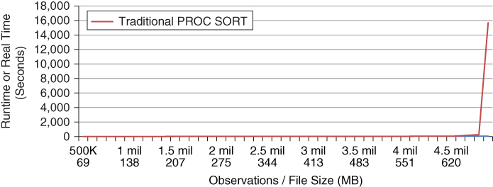
Figure 8.2 Inefficiency Elbow Caused by RAM Exhaustion
Figure 8.2 demonstrates an inefficiency elbow typical of decreasing available memory, where executions to the left of the elbow demonstrate efficiency in use and executions to the right of the elbow demonstrate inefficiency in use and a failure of scalability. But the executions to the right of the elbow also demonstrate inefficient software—not because of increased memory utilization, but because of the increase in I/O functions required to accommodate the restricted memory environment. Thus, the number of page faults—demonstrated through FULLSTIMER metrics in UNIX environments—represents I/O usage and increases dramatically beyond the inefficiency elbow. Not all SAS processes will experience an inefficiency elbow since some processes terminate with a failure rather than switching to virtual memory. Only through stress testing, described in the “Stress Testing” section in chapter 16, “Testability,” can SAS practitioners understand both performance failure and functional failure patterns of software.
I/O Processing
I/O processing requires resources to read and write data to disk. I/O processing is often commingled with CPU cycles and memory and may be difficult to disentangle. One clear way to differentiate time spent processing I/O requests versus computational tasks is to utilize the _NULL_ option in a DATA step that has no other input or output. Thus, the DATA step demonstrated in the “CPU Processing” section is reprised here; however, no output is created and the number of observations has been increased to 1 billion:
data _null_;
   length num1 8;
   do i=1 to 1000000000;
      num1=rand('uniform'),
      output;
      end;
run;
NOTE: DATA statement used (Total process time):
      real time           36.48 seconds
      user cpu time       34.85 seconds
      system cpu time     0.03 seconds
      memory              750.31k
      OS Memory           32888.00k
With no I/O operations required by the _NULL_ option, the computations complete in only 36 seconds, with CPU time taking approximately only 35 seconds, thus representing efficient execution of the code:
data sortme (drop=i);
   length num1 8;
   do i=1 to 1000000000;
      num1=rand('uniform'),
      output;
      end;
run;
NOTE: DATA statement used (Total process time):
      real time           8:32.74
      user cpu time       1:26.56
      system cpu time     8.25 seconds
      memory              751.59k
      OS Memory           32888.00k
However, when I/O operations are required to write the Sortme data set, the CPU time takes four times longer to process, demonstrating that three-quarters of the CPU resources reflect I/O processing (writing the data set), while only 35 seconds (or one-quarter) of CPU resources were used to create the data set. Moreover, note that the efficiency of CPU resources plummeted when I/O processing was incorporated—from 95.6 percent (or 34.9 seconds / 36.5 seconds) to 18.5 percent (or 1 minute 34.8 seconds / 8 minutes 32.7 seconds).
To provide one final example, now that the Sortme data set has been created, it can be used to assess the relative performance of input operations. The following code reads the Sortme data set but writes no output file and performs no other operations:
data _null_;
set sortme;
run;
NOTE: There were 1000000000 observations read from the data set WORK.SORTME.
NOTE: DATA statement used (Total process time):
      real time           1:35.14
      user cpu time       46.03 seconds
      system cpu time     5.95 seconds
      memory              953.21k
      OS Memory           10472.00k
CPU time required only 52.0 seconds for the task, but real time required one minute 35.1 seconds, almost twice as long. These performance metrics help demonstrate not only the cost of input operations but also the relative inefficiency. These examples provide a clear indication that software performance (on this system) could be increased through programmatic endeavors to decrease I/O processing, and through nonprogrammatic purchase of hardware to facilitate faster I/O processing. As a general rule, the extent to which reading and writing data sets—especially large ones—can be minimized will significantly improve performance.
Disk Space
Whereas I/O processing represents the speed with which data are written to or read from some location, disk space demonstrates the total storage required by some process. Disk space is differentiated because specific SAS runtime errors occur when SAS runs out of disk space, causing failure. Although some environments may be limited by disk space, due to the decreasing cost of storage, this resource limitation is becoming increasingly uncommon. Still, as the cumulative quantity of data continues to increase in organizations, disk space is a resource that shouldn't be ignored.
When SAS does run out of disk space, it produces a series of runtime errors, as demonstrated in the following output:
proc sort data=perm.bigdata out=perm.sorted;
   by char1;
run;
ERROR: No disk space is available for the write operation.  Filename =
       C:UsersmeAppDataLocalTempSAS Temporary
       FilesSAS_util0001000003CC_comput03CC000029.utl.
ERROR: Failure while attempting to write page 1352 of sorted run 15.
ERROR: Failure while attempting to write page 44934 to utility file 1.
ERROR: Failure encountered while creating initial set of sorted runs.
ERROR: Failure encountered during external sort.
ERROR: Sort execution failure.
NOTE: The SAS System stopped processing this step because of errors.
NOTE: There were 80493346 observations read from the data set SAFESORT.BIGDATA.
WARNING: The data set SAFESORT.SORTED may be incomplete.  When this step was stopped there were 0 observations and 10 variables.
NOTE: PROCEDURE SORT used (Total process time):
      real time           9:55.38
      cpu time            2:15.97
In this example, SAS has created utility files—temporary files that the SORT procedure uses to perform multithreaded sorting—but the cumulative size of those files (which are saved by default to the WORK library) has exceeded the allowable size of the WORK library. A full WORK library is one of the most common sources of disk space errors and can occur for several reasons:
- Failure to delete contents of WORK between SAS programs
- Extremely large data sets saved to WORK
- Iterative DATA steps saving incrementally named data sets to WORK
- Utility files, the behind-the-scenes temporary files created by SAS
I grew up in a house with a septic tank; you typically don't realize it's full until it's too late, there's a telltale stench emanating from the yard, and the lawnmower starts sinking into brown puddles. The SAS WORK library operates similar to a septic tank and won't give any indication it's approaching its capacity—only when it's full. But despite the lack of warning, there are steps that can be taken to lessen the likelihood of an overflowing disk. One of the simplest solutions is to delete the entire WORK library before or after usage with either the DATASETS or DELETE procedure.
When large data sets are saved to the WORK library, WORK will need to be deleted more often—sometimes multiple times within a single program. This can also occur when software iteratively creates numerous successive data sets in the WORK library in the process of creating some permanent data set. For example, the following development pattern is common (yet not always advisable) within SAS software:
data temp1;
   * read/create data;
run;
data temp2;
   set temp1;
   * transform data;
run;
data temp3;
   set temp2;
   * transform data;
run;
The development pattern is common because it allows a SAS practitioner to inspect data sets throughout successive processes and because it facilitates manual recreation of later data sets from earlier data sets if errors necessitate that data must be recreated. At the very least, when the ultimate data set in the sequence finally is created (and validated), the prerequisite data sets should be deleted so they don't clutter the WORK library.
Another best practice that prevents the WORK library from filling up and that supports recoverability is to save temporary data sets instead to a shared library so that these can be used as checkpoints in the event of software failure. This is discussed and demonstrated in the “Rerun Program” section in chapter 5, “Recoverability.” For example, data could be saved to PERM.Temp2 (rather than WORK.Temp2), enabling automatic recovery from checkpoints given implementation of appropriate business rules. And, as before, once the final data set is created (and validated), the incrementally named “Temp” data sets can be deleted from the PERM library to minimize disk space usage.
If these commonsense solutions to reducing disk space usage in the WORK library still fail to produce desired results, the WORK library can be permanently associated to a new disk volume. And for disk space errors occurring outside the WORK library, purchasing additional storage is the obvious solution.
Personnel
The time that SAS practitioners spend developing software is a software development resource that should be associated with project or software development costs, but should not be considered an operational resource. However, when personnel are responsible for manually executing software, validating SAS logs, or performing other manual operational functions, this time does represent resource utilization and can be considered when assessing the overall efficiency of a software product. This underscores the importance of software automation as the final step in building production software. Removing the human element from operational software can tremendously improve performance and efficiency, freeing developers to pursue developmental activities rather than repetitive, operational tasks.
EFFICIENCY IN THE SDLC
The most important decision about the role of efficiency in the SDLC is whether to require or monitor efficiency at all. As demonstrated, efficiency is more complex than assessing execution time or CPU time. Moreover, because CPU time, memory, I/O processes, disk usage, and personnel use different units of measurement, it's difficult to provide a multivariate solution that weighs components against each other, let alone that includes multiple resources. For example, if a SAS process is modified so that it uses less memory but now requires more CPU cycles, has it been made more or less efficient? That will ultimately depend on how individual resources are valued by stakeholders.
The value of resources can vary between organizations and stakeholders; over time, as hardware or infrastructure is updated, resource valuation can vary even within an organization. For example, large SAS grid environments may exemplify processing power that feels limitless and that represents a threshold that would be difficult for SAS processes to exceed. In such an environment, SAS practitioners might largely ignore CPU time in efficiency calculations or considerations because of its seemingly limitless capacity. Thus, efficiency might be defined uniquely by each organization or team based on relative resource value, real constraints, imposed limitations, and the overall effect on other performance attributes such as execution speed.
Given the complexity of the multivariate relationships inherent in resource utilization and optimization, the most common method to tackle the efficiency conundrum is to use software execution time as the primary performance metric for efficiency. However, in assessing software speed, it's important to understand the resources that collectively can make software faster or slower and to interrogate these resources individually to drive higher performing software.
Requiring Efficiency
For better or for worse, efficiency requirements are commonly referenced in terms of execution time alone with no mention of resource utilization. An awareness of resource utilization, however, is required—otherwise you're measuring only speed, not efficiency. Thus, requirements for efficiency can reference execution time but must also reference system resource utilization. Where this misnomer exists, requirements documentation should be amended to represent the true quality characteristic that is being discussed, required, or measured—whether speed or efficiency.
For example, consider the customer who specifies only that a SORT procedure must complete in less than ten minutes, but fails to specify any actual efficiency requirements or constraints. The savvy SAS practitioner could sneak out, buy a faster processor, and deliver software that meets this solitary requirement. The process still might consume identical resources, but could complete much faster, thus tremendously improving execution efficiency but not efficiency. Another SAS practitioner might instead perform six simultaneous sorts in parallel, thus implementing a divide-and-conquer technique to achieve several sorted data sets that are subsequently merged into a composite sorted data set. This solution would also be wicked fast, but would consume more resources in a limited time period, thus possibly monopolizing system resources. Again, this solution would also improve execution efficiency, but would actually decrease efficiency due to the increased use of resources.
In each case, the SAS practitioner would have delivered the required speed requirement, but may also have incurred unintended consequences related to resource utilization. In the first example, the cost of new hardware represents additional project (not operational) resources that the customer might not have intended to purchase. In the second example, the monopolization of resources could cause other processes to run slowly or fail if the additional processing power and memory were not available when requested. Thus, efficiency metrics can be required to specify resource utilization thresholds that software should not exceed.
Resource Exception Handling
It can be difficult to estimate CPU, memory, I/O, or disk space usage in planning or design phases, and often these resources can be reliably assessed only once software has been developed. Thus, rather than trying to stab in the dark and risk describing inaccurate resource utilization metrics in requirements documentation, a better approach is to briefly state a commitment to resource monitoring and governance to support robustness and fault-tolerance against resource overuse or exhaustion.
For example, if load and stress testing have demonstrated that a SORT procedure begins to perform inefficiently as the file size approaches 1 GB, a useful requirement might state that file size must not exceed 900 MB, that file size will be dynamically monitored by software, and that exception handling will proactively and automatically split larger files and sort them using divide-and-conquer techniques to prevent inefficient performance. While the 1 GB limitation most likely would not be known during software planning, a proxy value could be used to demonstrate the intent to develop software that will be robust to diminished resources. As development teams become more aware of their specific environments and respective resource utilization and limitations, they can become eerily accurate at predicting resource utilization even in planning and design phases. Data governors that can automatically detect and handle exceptionally large data are discussed in the “Data Governor” section in chapter 9, “Scalability.”
When SAS processes are executed, both FULLSTIMER and NOFULLSTIMER SAS logs demonstrate real time and CPU time, thus enabling a rough estimate of process efficiency to be gauged by dividing the latter into the former. Monitoring this quotient will not demonstrate programmatic efficiency—whether the software is efficiently coded—but can provide an indication of how efficiently the process is executing in the environment. Thus, monitoring these performance metrics over time (by automatically collecting, saving, and analyzing SAS logs) can be used to isolate processes that more often execute inefficiently. Armed with this information, SAS practitioners can highlight processes that are relatively less efficient and can implement either programmatic solutions to improve the performance of those specific processes, or nonprogrammatic solutions to improve the infrastructure as a whole.
Limit Parallel Processing
I once introduced the concept of parallel processing to a SAS team, and in about a month the server was in need of a serious laxative—nothing could get through it no matter how hard we pushed. Even with a small team, we had so many processes running simultaneously that we had effectively used the server's entire bandwidth. While parallel processing, described in chapter 7, “Execution Efficiency,” and chapter 12, “Automation,” should be implemented where software requires expedited processing, SAS practitioners must be cautioned that this concentrates resource utilization and can overwhelm the infrastructure.
When we met to discuss how and why the server was suddenly failing, we discovered that nearly everyone had converted SORT procedures and other processes to run in parallel across sometimes six or more SAS sessions! And, when these parallel processes were running concurrently with other parallel processes, it appeared to the SAS server as though our team size had suddenly quadrupled or sextupled overnight. Although parallel processing is one of the most effective methods to boost execution efficiency, it does not increase efficiency and, if implemented injudiciously, can stall or crash a SAS server. Thus, in some instances, requirements documentation may actually need to explicitly prohibit or limit parallel processing.
For example, in SAS environments that suffer from very real resource constraints, I've encountered teams that limit parallel processing during core business hours (i.e., when the server is more likely to be hit with manually executed jobs) by restricting SAS practitioners to one, two, or three sessions. Thus, you could run a three-pronged divide-and-conquer sort, or you could execute three separate analytic routines, but don't you dare run them all at once. A more exact yet less tenable approach might be to describe the maximum amount of resources that a SAS practitioner should be using at any one time. But, since a valid and useful requirement must be measurable, this more exact solution is often a better theoretical construct to be used for anticipating server load than for actually limiting resource utilization. Moreover, as production software is stabilized, automated, and scheduled, these jobs—which may over time account for the majority of SAS server bandwidth—are run administratively, rather than from user accounts.
Measuring Efficiency
System resources are most effectively measured programmatically with the FULLSTIMER SAS system option, which provides more performance metrics than the default NOFULLSTIMER option. The following example demonstrates FULLSTIMER invoked within the SAS Display Manager for Windows, depicting execution time (real time), CPU time, and memory usage but not I/O resource utilization:
options fullstimer;
data perm.sortme (drop=i);
   length num1 8;
   do i=1 to 1000000000;
      num1=rand('uniform'),
      output;
      end;
run;
NOTE: The data set PERM.SORTME has 1000000000 observations and 1 variables.
NOTE: DATA statement used (Total process time):
      real time           2:32.63
      user cpu time       1:29.57
      system cpu time     6.81 seconds
      memory              751.59k
      OS Memory           32888.00k
      Timestamp           04/18/2016 10:40:42 PM
      Step Count                        132337  Switch Count  0
A benefit of SAS performance metrics written to the log is their robustness to software failure. If a process terminates prematurely with an error, FULLSTIMER metrics are still produced that demonstrate resource utilization up to the point of failure. This is beneficial when failures occur due to resource-related runtime errors, such as the infamous out-of-memory error. By saving FULLSTIMER metrics to an external file and monitoring that file for not only resource utilization but also runtime errors, SAS practitioners can pinpoint resource utilization levels when failures occur. Awareness of critical resource utilization thresholds is necessary when implementing data governors, as discussed in the “Data Governors” section in chapter 9, “Scalability.”
FULLSTIMER System Option
FULLSTIMER metrics vary by SAS environment, with Windows environments providing far fewer metrics than UNIX environments. Because the SAS University Edition runs on LINUX, when the previous code is executed (on the same box with identical system resources, albeit from this different SAS interface), it produces the following output:
options fullstimer;
data perm.sortme (drop=i);
   length num1 8;
   do i=1 to 1000000000;
      num1=rand('uniform'),
      output;
      end;
run;
NOTE: The data set PERM.SORTME has 1000000000 observations and 1 variables.
NOTE: DATA statement used (Total process time):
      real time           3:48.17
      user cpu time       2:00.22
      system cpu time     17.82 seconds
      memory              786.28k
      OS Memory           26780.00k
      Timestamp           04/20/2016 06:36:33 AM
      Step Count                        9  Switch Count  46
      Page Faults                       0
      Page Reclaims                     386
      Page Swaps                        0
      Voluntary Context Switches        489961
      Involuntary Context Switches      737
      Block Input Operations            0
      Block Output Operations           8
Not only are additional metrics available, but also note the slower performance and significantly increased CPU utilization within SAS University Edition as compared with the SAS Display Manager for Windows. In most cases, software development and optimization occurs on a single system, so FULLSTIMER metrics will be consistently represented. However, as demonstrated in the “Contrasting the SAS University Edition” section in chapter 10, “Portability,” significant differences exist between the performance of the SAS University Edition and other SAS interfaces, which can be demonstrated through FULLSTIMER metrics.
In the next example, a subset of the 1 billion-observation Sortme data set is created, but the WHERE option is mistakenly placed in the DATA step statement rather than the SET statement. This requires the SET statement to read all observations, after which only approximately 10 percent are output to the Subset data set:
data perm.subset (where=(num1<.1));
   set perm.sortme;
run;
NOTE: There were 1000000000 observations read from the data set PERM.SORTME.
NOTE: The data set PERM.SUBSET has 99994212 observations and 1 variables.
NOTE: DATA statement used (Total process time):
      real time           9:46.37
      user cpu time       2:38.26
      system cpu time     6.33 seconds
      memory              961.18k
      OS Memory           32888.00k
The revised code produces the same functionality, but more efficiently places the WHERE option in the SET statement, thus only reading approximately 10 percent of the Subset data set. Efficiency is improved due to the reduced CPU cycles required, but because the variable Num1 still has to be interrogated to determine if each observation should be included, memory consumption remains identical between the two methods:
data perm.subset;
   set perm.sortme (where=(num1<.1));
run;
NOTE: There were 99994212 observations read from the data set PERM.SORTME.
      WHERE num1<0.1;
NOTE: The data set PERM.SUBSET has 99994212 observations and 1 variables.
NOTE: DATA statement used (Total process time):
      real time           6:57.14
      user cpu time       56.58 seconds
      system cpu time     9.93 seconds
      memory              961.59k
      OS Memory           32888.00k
Although not demonstrated in the SAS Display Manager output, when the two methods are compared in the SAS University Edition, the more efficient solution also clearly demonstrates the reduced I/O resources utilized, given that only 10 percent of the data were ingested into the data set. The inefficient code requires almost twice as many page reclaims. However, if a SAS practitioner were not aware of the best practice of including the WHERE option in the SET statement (as opposed to the DATA step statement), he might have considered the first solution efficient. Thus, when optimizing SAS software, a solution often isn't considered inefficient until it is outperformed either in theory or practice.
This underscores the relativity of measuring and assessing efficiency. Solutions are rarely decried as “the most efficient way ever” but rather as “more efficient,” “less efficient,” or “efficient enough.” Thus, if the first (inefficient) solution were in use in SAS software, and stakeholders were pleased with the software's performance and efficiency, it probably wouldn't be judged as inefficient because it met the business need. However, when compared to the second (optimized) code, it is evident that the first solution is relatively inefficient compared to the second because it fails to incorporate the SAS software development best practice of WHERE placement.
FULLSTIMER Automated
A common goal of production software is to maximize operational efficiency by removing the human element and automating SAS jobs. When software is automated, log parsing (and validation) also should be automated to eliminate tedious, error-prone, manual review of the SAS log. Numerous texts demonstrate automated methods to parse SAS logs, thus freeing SAS practitioners to pursue more creative and meaningful endeavors. Most examples in literature, however, use the PRINTTO procedure to write the entire log to a text file, after which it is parsed when software terminates. For many purposes, this is sufficient; however, it does not enable dynamic processing based on log results.
A second goal of production software is often to embed an exception handling framework that aims to increase the robustness and fault tolerance of software through dynamic, data-driven, fuzzy logic. For this reason, FULLSTIMER metrics might need to be accessed immediately after a process has completed so they can dynamically alter program flow (if needed). For example, if FULLSTIMER detects that a process used too much memory or that the ratio of CPU time to execution is below some established threshold, program flow can be altered due to inefficient or overutilization of system resources, by sending an alert email to stakeholders, by automatically terminating lower-priority jobs, or through other methods.
The following %READFULLSTIMER macro ingests a text file that includes FULLSTIMER log output and subsequently assigns global macro variables to values found in the FULLSTIMER metrics. For example, when “real time” is detected in the file, the global macro variable &REALTIME is assigned to the value. Because some UNIX FULLSTIMER metrics are not available in the Windows environment, missing metrics are assigned a value of –9:
%macro readfullstimer(textfile=);
* converts all times to seconds SS.xx format from HH:MM:SS.ss format;
%let syscc=0;
%global fullstimerRC;
%global realtime;
%global usercputime;
%global systemcputime;
%global memory;
%global osmemory;
%global stepcount;
%global switchcount;
%global pagefaults;
%global pagereclaims;
%global volcontextswitches;
%global involcontextswitches;
%global blockinops;
%global blockoutops;
%global errtextlong;
%let fullstimerRC=;
%let realtime=;
%let usercputime=;
%let systemcputime=;
%let memory=;
%let osmemory=;
%let stepcount=;
%let switchcount=;
%let pagefaults=;
%let pagereclaims=;
%let volcontextswitches=;
%let involcontextswitches=;
%let blockinops=;
%let blockoutops=;
%let errtextlong=;
data _null_;
length tab $100 errtextlong $2000 erryes 8;
infile "&textfile" truncover;
input tab $100.;
if _n_=1 then errtextlong='';
if _n_>=5 then do; *** needs to be made dynamic based on which
version of FULLSTIMER is used;
if find(tab,"ERROR")>0 or find(tab,"WARNING")>0 then erryes=1;
else if find(tab,"real time")>0 then erryes=0;
if erryes=1 then errtextlong=strip(errtextlong) || ' *** ' ||
strip(tab);
call symput('errtextlong',strip(errtextlong));
if lowcase(substr(tab,1,9))='real time' then do;
if count(scan(substr(tab,10),1,' '),':')=0 then call
symput('realtime',scan(substr(tab,10),1,' '));
else if count(scan(substr(tab,10),1,' '),':')=1 then call
symput('realtime',(input(strip(scan(substr(tab,10),
1,':')),8.0) * 60) +
input(strip(scan(substr(tab,10),2,':')),8.2));
else if count(scan(substr(tab,10),1,' '),':')=2 then call
symput('realtime',(input(strip(scan(substr(tab,10),
1,':')),8.0) * 3600) +
(input(strip(scan(substr(tab,10),2,':')),8.0) * 60) +
input(strip(scan(substr(tab,10),3,':')),8.2));
end;
else if lowcase(substr(tab,1,13))='user cpu time' then do;
if count(scan(substr(tab,14),1,' '),':')=0 then call
symput('usercputime',scan(substr(tab,14),1,' '));
else if count(scan(substr(tab,14),1,' '),':')=1 then call
symput('usercputime',(input(strip(scan(substr(tab,14),
1,':')),8.0) * 60) +
input(strip(scan(substr(tab,14),2,':')),8.2));
else if count(scan(substr(tab,14),1,' '),':')=2 then call
symput('usercputime',(input(strip(scan(substr(tab,14),
1,':')),8.0) * 3600) +
(input(strip(scan(substr(tab,14),
2,':')),8.0) * 60) +
input(strip(scan(substr(tab,14),3,':')),8.2));
end;
else if lowcase(substr(tab,1,15))='system cpu time' then do;
if count(scan(substr(tab,16),1,' '),':')=0 then call
symput('systemcputime',scan(substr(tab,16),1,' '));
else if count(scan(substr(tab,16),1,' '),':')=1 then call
symput('systemcputime',(input(strip(scan(substr(tab,16),
1,':')),8.0) * 60) +
input(strip(scan(substr(tab,16),2,':')),8.2));
else if count(scan(substr(tab,16),1,' '),':')=2 then call
symput('systemcputime',(input(strip(scan(substr(tab,16),
1,':')),8.0) * 3600) +
(input(strip(scan(substr(tab,16),2,':')),8.0) * 60) +
input(strip(scan(substr(tab,16),3,':')),8.2));
end;
else if lowcase(substr(tab,1,6))='memory' then call
symput('memory',scan(substr(tab,7),1,' k')/1024); *convert
KB to MB;
else if lowcase(substr(tab,1,9))='os memory' then call
symput('osmemory',scan(substr(tab,10),1,' k')/1024);
*convert KB to MB;
else if lowcase(substr(tab,1,10))='step count' then do;
call symput('stepcount',scan(substr(tab,11),1,' '));
call symput('switchcount',scan(substr(tab,11),4,' '));
end;
else if lowcase(substr(tab,1,11))='page faults' then call
symput('pagefaults',scan(substr(tab,12),1,' '));
else if lowcase(substr(tab,1,13))='page reclaims' then call
symput('pagereclaims',scan(substr(tab,14),1,' '));
else if lowcase(substr(tab,1,26))='voluntary context switches'
then call symput('volcontextswitches',scan(substr(tab,27),
1,' '));
else if lowcase(substr(tab,1,28))=
'involuntary context switches' then call
symput('involcontextswitches',scan(substr(tab,29),1,' '));
else if lowcase(substr(tab,1,24))='block input operations' then
call symput('blockinops',scan(substr(tab,25),1,' '));
else if lowcase(substr(tab,1,25))='block output operations'
then call symput('blockoutops',scan(substr(tab,26),1,' '));
end;
retain erryes errtextlong;
run;
* set all missing values to -9;
%let macrolist=realtime usercputime systemcputime memory osmemory
stepcount switchcount pagefaults pagereclaims volcontextswitches
involcontextswitches blockinops blockoutops;
%let i=1;
%do %while(%length(%scan(¯olist,&i,,S))>1);
%let mac=%scan(¯olist,&i,,S);
%put MAC: &mac &&&mac;
%if %length(&&&mac)=0 %then %let &mac=-9;
%let i=%eval(&i+1);
%end;
%let errtextlong=%sysfunc(compress("&errtextlong",,kns));
%if &syscc>0 %then %do;
%let fullstimerRC=FAILURE;
%return;
%end;
%mend;For example, to implement the %READFULLSTIMER macro on the DATA step that creates PERM.Subset, the following code is executed.
libname perm 'c:perm';
%let path=%sysfunc(pathname(perm));
options fullstimer;
proc printto log="&path/out.txt" new;
run;
data perm.subset;
   set perm.sortme (where=(num1<.1));
run;
proc printto;
run;
%readfullstimer(textfile=&path/out.txt);
Because the SAS log is saved to an external file Out.txt, and because that file may be repetitively overwritten by successive invocations of %READFULLSTIMER, exception handling inside the %READFULLSTIMER macro captures runtime errors that may occur. Given this framework, software can respond dynamically to real-time resource utilization by assessing the global macro variables that are created. These global macro variables can also be saved in a historical data set for longitudinal analysis of software performance.
WHAT'S NEXT?
Execution efficiency and efficiency describe rapid performance and appropriate utilization of system resources. But in data analytic environments, often the greatest source of variability in production software are the data themselves. As data volume or velocity increase, the performance and efficiency of software can wane, demonstrating a lack of scalability. chapter 9, “Scalability,” demonstrates scalable software that supports increased data volume, demand, and hardware infrastructure.