Chapter 7
Execution Efficiency
Following my first tour of duty in Afghanistan, I moved to Antigua, Guatemala, to unwind and relax for a few months. One of the most cosmopolitan cities in Central America, Antigua's fabled cobblestone streets are lined with backpacker hostels, quaint cafés, international cuisine, and 17th- and 18th-century cathedrals and colonial architecture, all laid beneath the volcanos Agua, Fuego, and Acatenango.
I'd visited Antigua years before with a friend and, flying into Guatemala City some 26 miles from Antigua, we'd hailed a cab to the bus exchange where we'd caught a chicken bus to Antigua. Aside from the conductor (driver) yelling at us at one point to put our heads down (possibly a bad part of town?), it was an uneventful yet laboring hour-long journey winding through the mountains, making stop after stop.
Now living in Antigua, as friends and family would fly in and out of Guatemala City to visit, I'd meet them at the airport, and we'd typically catch a shared shuttle back to Antigua, one of the fastest methods since it bypassed the central terminal and made no extra stops.
But, in first getting from Antigua to the city to pick them up, I had several options. When running extremely late, I called a private cab I knew to be very reliable; if available, he'd race over and ferry me to the city in the fastest possible manner.
Shared shuttles were the next-fastest method, but departed on predetermined schedules primarily from Parque Central (the central plaza). Because seats filled up quickly, tickets generally had to be purchased in advance.
For a more leisurely but jostling journey, “express” chicken buses ran from the Antigua terminal to the Guatemala City terminal, from which taxis ran to the airport.
And, for the slowest possible journey, local chicken buses made frequent stops through the 26-mile course, taking nearly 90 minutes. But the stops also provided opportunities for shopping or to take in a movie at the mall on the way.
While speed was typically the deciding factor for choosing one conveyance over another, other factors did exist. Each method had its own price, with taxis being the most expensive and local chicken buses the cheapest. Although I never encountered any threats, shared buses were touted as the safest method. And, while slower and less comfortable, chicken buses always provided the best stories and most memorable encounters with the Guatemalan people—and their livestock!

When I made a decision to take one transportation modality over another based solely on the expected duration of travel, I was relying on a single constraint—execution efficiency, or speed. Software development stakeholders also typically want the fastest possible software, which can be achieved through both programmatic and nonprogrammatic endeavors.
But in traveling within Guatemala, the ability to make an isolated decision based solely on one factor (speed) was facilitated by the lack of influence of other constraints, including cost, comfort, security, and the adventure factor. Software operation also has competing constraints, with faster software often requiring more memory, input/output (I/O) processing, and CPU cycles. And merely because the constraints aren't considered in a decision doesn't eliminate them.
In assessing transportation cost, a local chicken bus was approximately $1, an “express” chicken bus $2, a shared shuttle $15, and a private taxi $30. To some backpackers who were truly pinching quetzales (Guatemalan currency), the price differential was significant enough to sway them toward chicken buses. This attitude is more common in software development environments, in which system resources do limit the speed with which processing can occur. A customer or SAS administrator is likely aware that he could procure more processing power or memory, but might not believe that faster processing justifies the expense.
In justifying their decision to transit solely on chicken buses, backpackers often stated that the chicken buses were more efficient than other methods—effectively assessing the speed of travel respective of the cost of resources, which amounted only to the bus fare. In software development, similarly, decisions often must be made not based solely on speed, but rather on software efficiency—or speed of processing respective of system resource utilization.
This chapter introduces execution efficiency, or throw-caution-to-the-wind speed, irrespective of the associated costs of system resources. The next chapter provides a contrast by focusing on efficiency, which evaluates processing speed respective of system resource utilization.
DEFINING EXECUTION EFFICIENCY
Execution efficiency is “the degree to which a system or component performs its designated functions with minimum consumption of time.”1 Efficiency, conversely, is “the degree to which a system or component performs its designated functions with minimum consumption of resources.”2 Execution efficiency (or software speed) examines the ability of software to perform effectively and quickly irrespective of system resource utilization, whereas efficiency does account for resources. This is an important distinction due to the frequent commingling of efficiency and speed in software discussion and literature.
Of all performance characteristics—dynamic and static—speed is most often discussed in SAS literature. Slower SAS software delays results, data products, and data-driven decisions from which business value is ultimately gained. Where time is money, those delays can incur real costs to stakeholders. Central to definitions of both efficiency and execution efficiency is the notion that a system must be functionally effective; therefore, developers must always ensure that software not only is fast but also is accurate.
This chapter aims to disentangle efficiency from execution efficiency, discussing software speed irrespective of system resource utilization. Rather than enumerating techniques widely described throughout SAS literature to make code faster, it introduces performance benefits that can be gained through modularized code, software critical path analysis, and parallel processing. For an understanding of software speed respective of resource utilization, chapter 8, “Efficiency,” demonstrates the relationship between software execution speed and resource utilization, including its critical role in facilitating software reliability.
FACTORS AFFECTING EXECUTION EFFICIENCY
If software speed is the dependent variable by which software performance so often is measured, then what are the independent variables? Some of the primary factors influencing software speed include:
- Hardware
- Network and infrastructure
- Third-party software
- SAS interface
- SAS version
- SAS options
- Software development best practices
- Data injects
SAS practitioners may have little to no influence over some of these factors, and it's common for developers only to be able to influence software speed programmatically through development best practices. For example, I've worked in research environments in which my computer had been purchased as part of a bulk order by the government. I had no control over our network, I had no influence over the SAS application modules that had been purchased, and I had no ability to upgrade our software to a new version of SAS. While these can be unfavorable development conditions if higher software performance is demanded, SAS practitioners in more restrictive environments are able to focus exclusively on software quality rather than exerting effort to learn and manipulate hardware, network, system, and other resources.
In other environments, however, SAS practitioners may be able to influence more aspects of their infrastructure. If they have the ability to purchase or upgrade hardware or SAS components, they will be able to achieve greater software performance. System resources can be levied to improve performance, such as by throwing additional CPUs, memory, or bandwidth at a problem. Although nonprogrammatic solutions are inherently costlier than programmatic ones, a tradeoff often exists because nonprogrammatic solutions can enable SAS practitioners to spend less time trying to finagle additional speed programmatically from a fixed infrastructure.
Another benefit of considering both programmatic and nonprogrammatic solutions to achieve greater speed is that while programmatic solutions often affect only one software product, an investment in system resources can buttress the infrastructure as a whole with improved hardware, software, or components. Additionally, like reliability and robustness, the fastest performing software will be delivered only by incorporating both programmatic and nonprogrammatic methods.
FALSE DEPENDENCIES
One of the hallmarks of data analytic software is that the code often reads as a novel, from cover to cover. In the beginning chapters, the code ingests some data, in later chapters the data are manipulated or transformed, and in final chapters a series of analyses is performed. Real dependencies exist because later processes rely on the completion of earlier processes; runtime errors that occur during ingestion can cascade into subsequent processes to cause failure, including runtime errors or, more egregiously, invalid data and data products. This phenomenon is discussed in the “Cascading Failures” section in chapter 6, “Robustness.”
As extract-transform-load (ETL) processes gain complexity, however, additional data sources, data volume, and data processes are often incorporated. Each of these aspects individually can contribute to false dependencies that occur when real prerequisites are not required but are nevertheless implemented through serialized code design. For example, a false dependency (of process) exists when a program first performs the MEANS procedure on a data set and subsequently performs the FREQ procedure:
data final;
   length char $10 num 8;
run;
proc means data=final;
   var num;
run;
proc freq data=final;
   tables char;
run;
In this example, the ordering of the code dictates that the FREQ procedure is performed after the MEANS procedure. However, the MEANS and FREQ procedures are in no way associated—each relies only on the Final data set. Moreover, because both the MEANS and FREQ procedures require only a shared lock on the Final data set, each procedure can in theory be performed in parallel. Thus, by restructuring the program flow to incorporate modular software design and by throwing more resources at the problem, a faster solution can be developed. The solution would not be more efficient—the net sum of resource utilization remains roughly identical—but it would demonstrate execution efficiency because it could be executed faster.
The following sections introduce critical path analysis, an analytic technique that can be used to remove false dependencies during design and development phases. In the later “Parallel Processing” section, theoretical critical path analysis is supplanted by demonstrations of techniques that implement parallel processing to achieve higher performing software. But before learning to run, the first step is crawling toward software modularity.
Toward Modularity
Modular software design is discussed throughout chapter 14, “Modularity,” but must begin with a description of what is not modular software. Monolithic—literally, single stone (from the Greek monos + lithos)—represents the common practice especially in procedural software languages of writing software comprised of single, large programs. The journey toward modularity (and inherently away from monolithic design) facilitates critical path analysis and subsequent parallel processing that can improve processing speed.
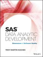
The critical path analysis model in Figure 7.1 demonstrates not only parallel MEANS and FREQ procedures, but also parallel Means and Freq modules. Software must first have the capacity to be divided into distinct modules so those modules can be relocated within the flowchart if beneficial. Only then can prerequisites, dependencies, inputs, and outputs be examined to start identifying and analyzing the critical path. Thus, while SAS data analytic software is often first envisioned as serialized processes that can be read like a novel, even novels are broken into discrete chapters. Could you imagine trying to parse this text if it weren't organized in some hierarchy that presented chapter, section, and subsection headings? It would not only be indecipherable to read but also would have been impossible to write!
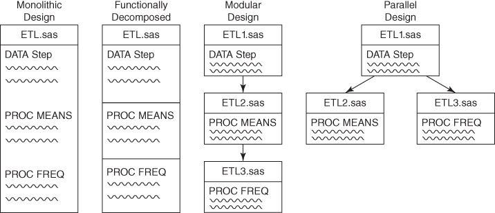
Figure 7.1 From Monolithic to Parallel Program Flow
The benefits of monolithic design in SAS are clear. Global macro variables can be easily passed throughout software if it comprises only one program. Initializations such as SAS library references also must be made only once in monolithic code. Code modules, on the other hand, each must be encapsulated and self-sufficient and, when they represent distinct SAS programs, must be passed parameters through the SYSTASK function, control tables, or other methods since macro variables cannot be passed between separate sessions of SAS. Despite the additional code complexity, modular software is preferred because it is more maintainable, readable, reusable, and testable, and—central to this chapter—faster. Figure 7.1 demonstrates the shift from monolithic to modular design, in which a quagmire of code is transformed from a single SAS program to three separate SAS programs.
Critical Path Analysis
Before exploring false dependencies, it's important to demonstrate a standardized methodology that can capture and display false dependencies. Due to the often serialized nature of data analytic software, flowcharts easily lend themselves to representing data processes. Flowcharts can be simple and temporary; whiteboards and Buffalo Wild Wings napkin sketches often achieve the same objective as enduring solutions like Visio or Microsoft Word SmartArt.
Flowcharting aims to identify inefficiencies in software design that can be corrected to produce faster software. In project management, critical path analysis similarly utilizes flowcharts to represent project activities and determine prerequisites, dependencies, inputs, and outputs. It can demonstrate which tasks can be performed in parallel to save time and which tasks might contribute to bottlenecks and ultimately project delays. More importantly, critical path analysis allows project managers to identify where to place or shift resources to achieve the greatest impact to increase throughput or reduce the project schedule.
To illustrate false dependencies hiding in monolithic software and the performance gains obtainable with modular, parallel program flow, the code in the “False Dependencies” section is demonstrated in Figure 7.2. While the FREQ procedure follows the MEANS procedure in the serialized code, in theory, both procedures could be run in parallel because each only requires completion of the DATA step (prerequisite) and because each only requires a shared lock on the Final data set (input).
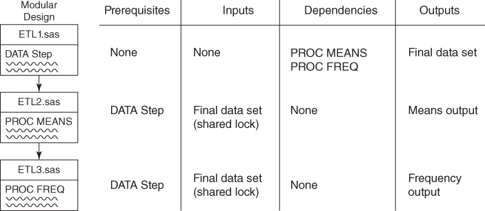
Figure 7.2 Critical Path Analysis
Assuming that the DATA step takes ten minutes to complete and the MEANS and FREQ procedures each take five minutes to complete, the serialized code would complete in 20 minutes, whereas the parallel code would execute in 15 minutes. Hooray, the software is more efficient! Or is it? In actuality, the system resources have not been reduced but only shifted so they are utilized concurrently. Although the software is faster, it is not more efficient.
Critical path analysis can be used to represent true prerequisites and true dependencies, thereby identifying and eliminating false dependencies—at least at the theoretical level. To enable SAS to run the MEANS and FREQ procedures in parallel, their respective code must be disentangled, modularized, and subtly redesigned as demonstrated in the following sections. The example demonstrated in Figure 7.2 is operationalized and automated in the “Synchronicity and Asynchronicity” section in chapter 12, “Automation.”
False Dependencies of Process
Dependencies of process occur when one process is reliant upon another, usually in which one process must complete before a subsequent process can begin. For example, in Figure 7.2, the MEANS procedure must wait until the DATA step ends, thus the MEANS procedure is a dependency of the DATA step. A false dependency, however, occurs when the serialized nature of software directs that two processes execute in series when they could in theory execute in parallel. Also demonstrated in Figure 7.2, the MEANS and FREQ procedures include a false dependency; each could complete in parallel because neither is dependent on the other and neither requires an exclusive lock on the Final data set.
One of the primary factors to consider in assessing process dependencies is the type of file lock that is required by a process. For example, the MEANS and FREQ procedures can execute at the same time because each requires only a shared—not exclusive—file lock on the Final data set. As a rule of thumb, whenever an exclusive lock is required by a module, that module cannot be performed concurrently with any other module requiring access to the same data set. For this reason, while fairly obvious, it's impossible to edit a data set (which requires an exclusive lock) while simultaneously analyzing the data set with the FREQ procedure.
False Dependencies of Data Sets
ETL processes are often efficiently designed to accommodate various types of throughput, such as processing three different transactional data sets on a daily basis. However, efficient software design (i.e., writing less code) can paradoxically contribute to slower software execution due to false dependencies that are created. In the following example, the transactional data sets One, Two, and Three are run through a single ETL process that contains distinct ingestion, transformation, and analysis functionality but that is coded through serialized design. The code prima facie may appear efficient because we've been conditioned to associate the SAS macro language with efficiency. After all, the %ETL macro can process a serialized list of data sets through the DSN parameter!
%macro ETL(dsn=);
* ingestion;
data &dsn;
   set &dsn._raw;
run;
* transformation;
data &dsn._trans;
   set &dsn;
run;
* analysis;
proc freq data=&dsn._trans;
   tables char;
run;
%mend;
%macro engine(dsnlist=);
%local i;
%let i=1;
%do %while(%length(%scan(&dsnlist,&i,,S))>1);
   %etl(dsn=%scan(&dsnlist,&i,,S));
   %let i=%eval(&i+1);
   %end;
%mend;
* required to fake ingestion streams;
data one_raw;
   length char $10;
data two_raw;
   length char $10;
data three_raw;
   length char $10;
run;
%engine(dsnlist=one two three);
This code demonstrates real dependencies in that the ingestion module must complete before the transformation module can start, and the transformation module subsequently must complete before the analysis module can start. The code also demonstrates false dependencies, however, in that it requires data set One to be processed before data set Two, and data set Two to be processed before data set Three. In reality, any or all of the modules processing data set One could fail (for example, if data set One had no observations) without negatively affecting the performance of data sets Two or Three. Figure 7.3 demonstrates the false dependencies formed when the ingestion of data set Two must wait for data set One to complete, and when the ingestion of data set Three must wait for data sets One and Two to complete.
Figure 7.3 Data Set False Dependencies
In theory, a faster solution would simultaneously ingest data sets One, Two, and Three, after which those three process flows would continue with their respective transformations and analyses. Figure 7.4 depicts the revised critical path, implementing parallel processing that removes all false dependencies. Note as before that this solution is not more efficient; however, it completes in approximately one-third the time of the original monolithic process flow.

Figure 7.4 Data Set False Dependencies Removed
False Dependencies of Throughput
The previous demonstrations have depicted software that can be modularized into smaller chunks to allow data sets to pass through them more quickly. Sometimes, however, the data set itself can be the source of the bottleneck if it is large and unwieldy. For example, consider a straightforward SAS SORT procedure that sorts 100 observations in less than a second:
data reallybig (drop=i);
   length num1 8;
   do i=1 to 100;
      num1=rand('uniform'),
      output;
      end;
run;
proc sort data=reallybig;
   by num1;
run;
But what happens to execution time when Reallybig actually is really big—say, 100 billion observations or 100 GB? This can present a scalability problem for some environments, causing slow or inefficient performance, or outright functional failure. The effect is similar to what happens when I throw a peeled orange into my koi pond—the koi and turtles quickly battle to get at the orange, completely surrounding it, but the smaller ones are pushed away, and even the larger ones can't nibble through to the center for over an hour. It's tremendously inefficient feeding. Yet when fish flakes are dumped in the pond, they're consumed in minutes because the koi and turtles all can be eating simultaneously. You similarly don't want to wait while your data analytic processes nibble their way to the center of a 100 GB orange!
The same phenomenon typically occurs in data processing, in which the first observation is processed, followed by the second, and so forth. When large data sets are encountered, however, performance can be improved by processing discrete segments of the data sets in parallel and thereafter reconstituting the data or results in a technique referred to as divide and conquer. In essence, parallel processing creates a feeding frenzy, allowing everyone to eat simultaneously and efficiently rather than waiting for a large mass to be consumed. The technique is described more fully in the “Load Scalability” section in chapter 9, “Scalability.”
For example, the following code represents the first module (of four) that would be run in parallel to sort the Reallybig data set with 100 observations:
proc sort data=reallybig (firstobs=1 obs=25);
   by num1;
run;
The second process (running in parallel) would sort observations 26 through 50, and so on. In this manner, all sorting would be done in parallel, after which those sorted data sets could be recombined for a potential performance improvement. This type of dynamic processing can be implemented with the SYSTASK statement, which can spawn batch jobs that execute in parallel. SYSTASK is demonstrated in the “Decomposing SYSTASK” section in chapter 12, “Automation.”
This divide-and-conquer technique can also be applied to DATA steps by processing different segments of observations in parallel. However, as with the SORT procedure, whenever data are divided they must later be recombined, which incurs additional processing time and resources. Because of this extra step, divide-and-conquer methods are always slightly less efficient than processing data as a single unit. However, when sufficiently large and despite this inefficiency, data sets can be processed much faster in parallel than as a single unit. Only through trial and error can thresholds be established to determine when and on what size data sets divide-and-conquer techniques will improve performance.
PARALLEL PROCESSING
By eliminating false dependencies, parallel processing can dramatically increase software speed by performing multiple tasks simultaneously. The previous “False Dependencies” section demonstrates how processes, data sets, and even observations can be decoupled and executed concurrently to increase performance. However, this increased speed typically decreases software efficiency. This occurs because parallel processing requires running multiple SAS sessions, each of which requires overhead resources. For example, when I start the SAS Display Manager, the Windows Task Manager depicts that SAS requires 57 MB of memory just to sit quietly and not even execute code.
A second source of inefficiency in parallel processing is the effort required to coordinate and communicate between SAS sessions. For example, if four SAS sessions are concurrently sorting 100 billion observations, some effort is required to determine which sessions will sort which specific chunks of observations. And each individual session should inform the other sessions once it completes sorting its chunk. A final step—not required for sorts performed on a single data set—is required to reconstitute the four data sets, thus utilizing even more resources. Each of these activities is costly, so while the parallel solution will never be more efficient, it will often be faster given sufficient resources (processors and memory) to perform the tasks.
One way to view parallel processing is that it allows developers to more fully utilize system resources. SAS environments with abundant or unused resources will benefit most fully from parallel processing because the processes effectively won't be in competition with each other. Even SAS practitioners running a single instance of the SAS Display Manager, however, can improve performance by more fully utilizing system resources through parallel processing.
No Multithreading Here!
Parallel processing is not multithreading! The distinction is made in the “Parallel Processing versus Multithreading” section in chapter 9, “Scalability,” but is underscored here. Throughout this text, parallel processing depicts processes and programs that run concurrently in separate SAS sessions. Whereas parallel processing typically only increases execution efficiency, multithreading often can also increase efficiency because it operates at the thread—not the process—level.
Hardcoded Concurrency
False dependencies between processes can be overcome through parallel processing that executes processes concurrently rather than in series. In some cases, this can be accomplished relatively easily, without much modification to the software and with little to no communication required between the individual SAS sessions. While hardcoded parallel processing solutions are uncommon in production software, they form the basis for later dynamic parallel design.
The previous “False Dependencies of Data Sets” section demonstrates the false dependency that exists when the data set One must pass through several phases of an ETL process before the data set Two can be processed. The inefficiency is caused by the invocation of the %ENGINE macro, because it requires a parameterized list of data sets that are processed in series.
%macro engine(dsnlist=);
%local i;
%let i=1;
%do %while(%length(%scan(&dsnlist,&i,,S))>1);
   %etl(dsn=%scan(&dsnlist,&i,,S));
   %let i=%eval(&i+1);
   %end;
%mend;
To overcome this inefficiency, the %ENGINE and %ETL macros don't even need to be modified—modifying only the %ENGINE invocation removes the serialization. For example, a SAS practitioner can open one SAS session and run the following code to process data set One:
%engine(dsnlist=one);And, in a separate SAS session, %ENGINE can be invoked only on data set Two:
%engine(dsnlist=two);The facile solution works fluidly because no further interaction between the data sets or their derivative processes is required. So long as resource utilization is not taxed by the second SAS session, the software should now process two data sets in the time previously required to process one.
A difficulty in implementing hardcoded solutions like this is that in production software, additional modifications are typically required. This code was substantially advantaged because the data set name was parameterized into the macro variable &DSN and utilized to dynamically create and name every referenced data set, ensuring that data sets from the first session did not conflict with or overwrite data sets from the second session. Data sets were also processed only in WORK libraries, whereas references to shared SAS libraries could have resulted in file access collisions. Finally, no interaction was required between the two sessions as they executed because no dependencies existed between either.
A hardcoded parallel processing solution can be easy to implement but very difficult to maintain because it requires developers or users to maintain separate code bases. For example, two separate macro invocations were required for %ENGINE, one to execute each of two data sets. Because the ultimate goal of production software is often to achieve stable software that can be scheduled, hardcoded parallel processing techniques generally have no place in production software. It is a useful tool to conceptually introduce parallel processing or to test software design, but hardcoded parallel design should typically be improved through dynamic, macro-driven software that does not require maintaining separate code bases.
Executing Software Concurrently
The “Hardcoded Concurrency” section demonstrates separate modules that can be run in parallel to achieve faster performing software. While this requires no communication between the sessions, more advanced parallel processing can execute multiple copies of the same program from separate sessions of SAS. This technique requires execution autonomy, because each software instance must coordinate with all others to ensure that duplication will not result. Moreover, it requires efficient and effective communication between all modules because they must report when they start a process, when they complete a process, and whether the process succeeded or failed.
To achieve execution autonomy, fuzzy business logic should prescribe prerequisites, dependencies, inputs, and outputs for each module. The following code, reprised from the earlier “False Dependencies” section, demonstrates that the FREQ procedure unfortunately must wait for the MEANS procedure to complete:
data final;
   length char $10 num 8;
run;
proc means data=final;
   var num;
run;
proc freq data=final;
   tables char;
run;
The DATA step process has no prerequisites, so it can execute immediately. The MEANS and FREQ processes each require the Final data set to have been created before they can start. After identifying prerequisites and dependencies and identifying that each process requires only a shared lock of the PERM.Final data set, it's clear (as depicted in Figure 7.2) that MEANS and FREQ can be run in parallel. The two procedures can be modularized through the following code, which is described later throughout the text:
%macro means();
%let start=%sysfunc(datetime());
%control_update(process=MEANS, start=&start);
proc means data=perm.final;
   var num;
run;
%lockitdown(lockfile=perm.control, sec=1, max=5, type=W, canbemissing=N);
%control_update(process=MEANS, start=&start, stop=%sysfunc(datetime()));
%mend;
%macro freq();
%let start=%sysfunc(datetime());
%control_update(process=FREQ, start=&start);
proc freq data=perm.final;
   tables char;
run;
%lockitdown(lockfile=perm.control, sec=1, max=5, type=W, canbemissing=N);
%control_update(process=FREQ, start=&start, stop=%sysfunc(datetime()));
%mend;
Communication is the next requirement to transition from monolithic to parallel design. Because global macro variables cannot be used to communicate between SAS sessions, a control table—a SAS data set—can be used to facilitate cross-session communication. In this example, one session will run the DATA step while the second session waits patiently for it to complete. Thereafter, upon detecting DATA step completion, one session will run the Means module while the other session runs the Freq module. Because both sessions must be able to access the Final data set and the control table, both data sets must be moved from the WORK library to a shared library.
* saved as c:permparallel.sas;
libname perm 'C:perm'; * modify to actual location;
%include 'C:permlockitdown.sas'; * modify to LOCKITDOWN location;
%macro control_create();
%if %length(&sysparm)>0 %then %do;
   data _null_;
      call sleep(&sysparm,1);
   run;
   %end;
%if %sysfunc(exist(perm.control))=0 %then %do;
   %put CONTROL_CREATE;
   data perm.control;
      length process $20 start 8 stop 8 jobid 8;
      format process $20. start datetime17. stop datetime17. jobid 8.;
   run;
   %end;
%mend;
%macro control_update(process=, start=, stop=);
data perm.control;
   set perm.control end=eof;
%if %length(&stop)=0 %then %do;
   output;
   if eof then do;
   process="&process";
   start=&start;
   stop=.;
   jobid=&SYSJOBID;
   output;
   end;
   %end;
%else %do;
   if process="&process" and start=&start then stop=&stop;
   %end;
   if missing(process) then delete;
   run;
&lockclr; * required by LOCKITDOWN macro;
%mend;
%macro ingest();
%let start=%sysfunc(datetime());
%control_update(process=INGEST, start=&start);
data perm.final;
   length char $10 num 8;
   do i=1 to 500000;
      do j=1 to 100;
         char=put(j,$10.);
         num=j;
         output;
         end;
      end;
run;
%lockitdown(lockfile=perm.control, sec=1, max=5, type=W, canbemissing=N);
%control_update(process=INGEST, start=&start, stop=%sysfunc(datetime()));
%mend;
%macro means();
%let start=%sysfunc(datetime());
%control_update(process=MEANS, start=&start);
proc means data=perm.final;
   var num;
run;
%lockitdown(lockfile=perm.control, sec=1, max=5, type=W, canbemissing=N);
%control_update(process=MEANS, start=&start, stop=%sysfunc(datetime()));
%mend;
%macro freq();
%let start=%sysfunc(datetime());
%control_update(process=FREQ, start=&start);
proc freq data=perm.final;
   tables char;
run;
%lockitdown(lockfile=perm.control, sec=1, max=5, type=W, canbemissing=N);
%control_update(process=FREQ, start=&start, stop=%sysfunc(datetime()));
%mend;
Because the control table PERM.Control is accessed by multiple sessions of SAS, and because an exclusive lock is required to update the data set, some quality control mechanism must ensure that file collision does not occur. The %LOCKITDOWN macro (or similar functionality) should be implemented before attempting to open the control table to ensure it is not in use. The %LOCKITDOWN macro first assesses the availability of a data set; if it is locked, the macro waits a parameterized amount of time before reattempting access. The %LOCKITDOWN macro is described more fully in chapter 9, “Scalability,” while the full text and code are available in a presentation titled “From a One-Horse to a One-Stoplight Town: A Base SAS Solution to Preventing Data Access Collisions through the Detection and Deployment of Shared and Exclusive File Locks.”3
The JobID variable in the control table records the unique value of the global macro variable &SYSJOBID. If run in series by a single session of SAS, the JobID will be identical for all processes. When run in parallel, however, the JobID will demonstrate the SAS session that ran each specific module. This information can be useful when trying to troubleshoot parallel processing to ensure that all sessions are executing. Table 7.1 demonstrates use of &SYSJOBID to determine whether parallel processing is running on all cylinders.
Table 7.1 Control Table Demonstrating Parallel Processing
| OBS | Process | Start | Stop | JobID |
| 1 | INGEST | 01JAN16:12:18:33 | 01JAN16:12:19:00 | 8040 |
| 2 | MEANS | 01JAN16:12:19:00 | 01JAN16:12:19:07 | 8040 |
| 3 | FREQ | 01JAN16:12:19:01 | 01JAN16:12:19:15 | 3100 |
The previous code demonstrates processes that create and update the control table, as well as that run the analytic macros MEANS and FREQ. In parallel processing design, however, an engine (AKA controller or driver) often includes the autonomous business logic that makes everything run—in this example, deciding whether to execute a module or sit and wait for other processes to complete. In production software, the engine will often operate as a separate program while spawning (or calling) child processes (batch jobs) saved as separate SAS programs. The following %ENGINE macro should also be included in the previous SAS program; the macro effectively controls and directs execution of separate SAS macros.
* continues the program c:permparallel.sas;
%macro engine();
%let ingest=;
%let means=;
%let freq=;
%control_create();
%do %until(&ingest=COMPLETE and &means=COMPLETE and &freq=COMPLETE);
   %lockitdown(lockfile=perm.control, sec=1, max=5, type=W,    canbemissing=N);
   data control_temp;
      set perm.control;
      if process='INGEST' and not missing(start) then do;
         if missing(stop) then call symput('ingest','IN PROGRESS'),
         else call symput('ingest','COMPLETE'),
         end;
      else if process='MEANS' and not missing(start) then do;
         if missing(stop) then call symput('means','IN PROGRESS'),
         else call symput('means','COMPLETE'),
         end;
      else if process='FREQ' and not missing(start) then do;
         if missing(stop) then call symput('freq','IN PROGRESS'),
         else call symput('freq','COMPLETE'),
         end;
   run;
   %if %length(&ingest)=0 %then %ingest;
   %else %if &ingest=COMPLETE and %length(&MEANS)=0 %then %means;
   %else %if &ingest=COMPLETE and %length(&FREQ)=0 %then %freq;
   %else %if &ingestˆ=COMPLETE or &meansˆ=COMPLETE or    &freqˆ=COMPLETE %then %do;
      &lockclr;
      data _null_;
         call sleep(1,1);
      run;
      %end;
   %else &lockclr;
   %end;
%mend;
%engine;
One hallmark of parallel software is its ability to be initialized from only one session of SAS. Thus, if only one session of the Parallel.sas program is executed, the software will execute in series. However, when multiple instances of the software are executed in separate SAS sessions, the programs will play nicely together because they communicate and coordinate program flow through the %ENGINE macro and the control table. As long as the second instance of the program is executed before the %MEANS macro has completed in the first SAS session, the second instance will access the control table and begin executing the %FREQ macro in parallel. While this example has demonstrated parallel processing that requires manual initialization of multiple SAS sessions and manual execution of multiple instances of the same program, in later sections, examples demonstrate parallel processing in which initialization and execution are automated via the SYSTASK statement.
Starting Concurrent SAS Sessions
The program Parallel.sas in “Executing Software Concurrently” was run manually, which necessitated multiple initializations of SAS sessions. Parallel processing can also be achieved by spawning clone child processes via SYSTASK, by spawning individual child processes via SYSTASK, or by executing batch programs (not batch jobs) from the operating system (OS)—each of which automatically creates concurrent SAS sessions. These methods are discussed more fully in chapter 12, “Automation,” while the “Demand Scalability” section in chapter 9, “Scalability,” discusses considerations and caveats when multiple instances of software are run simultaneously.
The entire code from the “Executing Software Concurrently” section should first be saved as C:permparallel.sas. A batch program or batch file—as opposed to a batch job—contains OS command line syntax and should be saved with the .bat extension. The following batch file (C:permseries.bat) can be created by opening Notebook or another text editor and entering the following syntax on only one line with no carriage returns:
"c:program filessashomesasfoundation9.4sas.exe" -sysin C:permparallel.sasThe location of the SAS.exe executable program may vary by SAS application and environment, and double quotes are required if its path contains a space, such as the “program files” folder. When the batch file is saved and subsequently executed, the SAS log is automatically saved to a log file—C:permparallel.log—because no log location is specified in the command statement. Before attempting to run the batch file in parallel, view the log to ensure that the program successfully ran in series. Once the log confirms that no runtime errors occurred, delete the PERM.Control and PERM.Final data sets to reset the session. If PERM.Control is not deleted, the program will correctly assess that the Ingestion, Freq, and Means modules all have completed, and thus will exit the software without rerunning any of these modules.
Once the software is confirmed to have run in series from the batch file, it can be tested in parallel. Once again, delete the PERM.Control and PERM.Final data sets to reset the session. The following batch file should be saved to C:permparallel.bat and, as before, the two commands should be on two separate lines without additional carriage returns:
start "job1" "c:program filessashomesasfoundation9.4sas.exe" ‐sysin "C:permparallel.sas" ‐log "C:permlog1.log" ‐print "C:permoutput1.lst" ‐sysparm 0
start "job2" "c:program filessashomesasfoundation9.4sas.exe" ‐sysin "C:permparallel.sas" ‐log "C:permlog2.log" ‐print "C:permoutput2.lst" ‐sysparm 5
The first line of the batch program initiates the first SAS session and runs the first instance of the Parallel.sas program. Without waiting for the first instance of the program to complete, the second line immediately (and asynchronously) initiates a second session of SAS and runs a second instance of the program. Because the default log and output files for each SAS program would have been identically named—as the same SAS program is being executed twice in parallel—unique log and output file names must be specified to avoid file collisions, which would cause errors.
The SYSPARM parameter passes a numeric value to the &SYSPARM automatic macro variable in the %CONTROL_CREATE macro, which waits a parameterized number of seconds before commencing. Without discrepant SYSPARM values—which allow the first instance of the program to build the control table immediately but force the second instance of the program to wait five seconds—each instance of the program would simultaneously assess that the control table did not exist and simultaneously attempt to build it, either overwriting each other or failing with file access errors. Thus, the first SAS session (and instance of the Parallel.sas program) will create the control table and run the DATA step, while the second instance of the program waits five seconds, assesses that the control table exists, and then enters a busy-waiting cycle until the DATA step completes and the control table is updated to reflect this. Thereafter, one session of SAS will execute the %MEANS macro while the other session executes the %FREQ macro.
The benefits of batch program design are numerous. The batch file can be used to launch multiple sessions of SAS automatically and run multiple SAS programs, rather than requiring SAS practitioners to initialize SAS sessions manually to open and run programs. Since batch files are run directly from the OS, they can be automated and scheduled to run through the OS, as discussed in the “Starting Batch from a Batch File” section in chapter 12, “Automation.” Most relevant to increased performance, batch files allow asynchronous and parallel processing that facilitates significantly faster software execution when code is modularized.
Naptime Is Inefficient
I was a huge fan of naptime as a kindergartener—we would each lie down on beach towels, spread across a large area rug, while Mrs. McCarthy read to us. In software development, however, naptime can be extremely inefficient. One of the only negative consequences of parallel software design is the busy-waiting (or spinlock) cycle that is often introduced to put a SAS session to sleep when it has nothing else to do. For example, when the batch file Parallel.bat in the “Starting Concurrent SAS Sessions” section executes, the program running in the second session enters a busy-waiting cycle while it waits for the DATA step to complete in the first session. During this naptime, despite only sleeping, the second SAS session is still consuming overhead system resources as well as additional resources used each time it queries the control table to determine whether the DATA step has completed. Thus, while parallel processing can perform significantly faster, these sleep cycles in part contribute to the lower efficiency demonstrated in parallel processing as compared to serial processing.
Serialized process flows, however, may run slowly, but they are always running—you won't catch a serialized program lying down on the job because it doesn't need to coordinate with or wait for external sessions or programs. While the overhead system resources utilized by a slumbering SAS session are minimal, when multiple SAS sessions are sleeping, or when SAS sessions spend an inordinate percentage of their lives in busy-waiting cycles due to poor management of parallel processes, the cumulative inefficiency can burden the overall SAS system.
While the %LOCKITDOWN macro will prevent failure associated with file access collisions, it will not prevent the associated delays inherent in parallel processing that occur when multiple SAS sessions vie for exclusive access to a single data set. If two SAS sessions simultaneously vie for exclusive access to a control table, the %LOCKITDOWN macro will ensure that one gains access to the data set while the other enters a busy-waiting cycle, rather than terminating with a runtime error. Access to control tables—which typically contain a few dozen to a few hundred observations—only requires a second or two and thus doesn't contribute to inefficiency. When complex processes are run on larger data sets, however, busy-waiting cycles can last hours, during which data accessibility is repeatedly tested at regular intervals.
Thus, in assessing performance gains experienced by parallel processing design, SAS practitioners should also assess potential inefficiency created by sleeping processes. The Parallel.sas program presented in the “Executing Software Concurrently” section, for example, is optimized when run on two SAS sessions because %MEANS can run in one session while %FREQ runs in the other. If run from three concurrent SAS sessions, however, the third program instance will sleep the entire time and add no value, thus further decreasing the software efficiency while not improving performance. Examination of control tables, as demonstrated in the following section, can help demonstrate when concurrent software is being run across an optimal number of SAS sessions.
Control Tables in Parallel Processing
Communication is the most important aspect of parallel processing because it enables individual SAS sessions to speak to each other to facilitate autonomous execution through fuzzy logic business rules. Communication ensures that prerequisites are met before processes begin and further ensures that redundant processing of the same tasks does not occur. Control tables should record when processes start (so that other instances don't accidentally start the same process), when processes complete (so that all instances are aware when prerequisite processes are finished), and when processes fail (so that the process can be restarted or have other actions taken, as well as to ensure that dependent processes do not start following the failure).
Table 7.1 demonstrates a control table from the Parallel.sas program in the “Executing Software Concurrently” section that shows successful completion of the software when run in parallel from two sessions of SAS. The control table demonstrates that the %MEANS and %FREQ macros ran in parallel, which can be assessed by examining start and stop times or by the separate SAS JobIDs, 8040 and 3100. Had only one JobID been listed, this would have indicated either that the software was executed from only one session or that other sessions had failed during execution. Had three sessions of SAS run three instances of the Parallel.sas program concurrently, only two JOB IDs would have been demonstrated since the third process would have had no tasks to complete, thus demonstrating the inefficiency of running three sessions.
EXECUTION EFFICIENCY IN THE SDLC
Software speed is a bit different than other performance requirements because it represents a continuous measurement rather than a dichotomous—successful or failed—outcome. For example, software may demonstrate a lack of robustness by terminating with a failure. Software that lacks portability may terminate with a failure when an unexpected (i.e., exceptional) environment is encountered. Thus, while failures associated with many other performance attributes can cause real functional failures, a failure of execution efficiency typically just describes slow execution. This can contrast with an efficiency failure, in which overuse of system resources can cause not only delays but runtime errors and loss of functionality.
Because execution efficiency lies on a continuum rather than existing as a dichotomous outcome, it can be prone to refactoring throughout the software development life cycle (SDLC), even once software is in production. For example, SAS practitioners may initially implement software that provides a functional outcome, but stakeholders may later require an increase in speed. Due to the vast number of methods that can be used to increase software speed—including programmatic and nonprogrammatic best practices—there are often multiple ways to achieve higher performing software over its lifespan. Because of this diversity, however, refactoring for increased speed is one of the most common requests from stakeholders for software already in production.
Requiring Execution Efficiency
This is an easy one—how long should the software take to complete? A typical requirement states only the maximum execution time; however, an average execution time might also be stated. Often in modular software design, in which modules are being independently developed by various SAS practitioners, individual modules will have their own performance requirements that state their respective execution time thresholds.
Because software speed is a continuous rather than discrete measurement, a common objective is to improve the speed of software throughout the SDLC, including once software is in production. I once encountered a customer who was astonished that a SAS process designed to be run hourly could not be compressed into 20 minutes without significant redesign and refactoring. Software quality represents an investment, and like other dimensions of quality, execution efficiency should be planned and implemented throughout the SDLC rather than in an ad hoc fashion once software has been completed. My team was eventually able to expedite the analytic process and run it in less than 20 minutes, but this required starting from scratch with a complete software overhaul. While customers may need to change software requirements drastically during or even after development, accurately conveying realistic software performance requirements during software planning and design will help eliminate later unnecessary redesign and refactoring.
Maximum Execution Time
When a maximum execution time is stated, it represents a standard that should never be exceeded—for example, “The ETL process will always complete in 20 minutes or less.” However, this simplistic efficiency requirement could allow developers to drain system resources, adversely affecting other processes. For example, to achieve this requirement, developers might design software that spawned 20 concurrent SAS sessions and overwhelmed a SAS server, preventing other unrelated programs from executing. Thus, a more comprehensive requirement might state: “The ETL process will always complete in 20 minutes or less while using no more than two processors concurrently and no more than 2 GB of memory.” The latter requirement incorporates both speed and efficiency and might be necessary in environments with many users or constrained system resources. In both examples, however, software that completes in 21 minutes represents a performance failure that should be documented and investigated.
Sometimes a maximum efficiency threshold is stated, but this standard can be exceeded on occasion. For example, a requirement might state that “The ETL process will complete in 20 minutes or less for 95 percent of executions, and 30 minutes or less for 5 percent of executions.” After all, requirements are intended both to guide design and development and to regulate function and performance, but should incorporate real-world variability that can exist. Thus, if SAS practitioners understand that on occasion, larger data sets will be processed that may slow execution speed and efficiency, this variability should be accounted for in software requirements. Another option is to state average execution time in requirements instead of (or in addition to) maximum execution time, thus providing a metric that more readily accommodates variability in run time.
Progressive Execution Time
Especially in Agile and other rapid software development environments, change is espoused and encouraged, and early delivery of functionality and business value is paramount. Thus, expecting customers to state or even know their ultimate performance objectives during early planning will be unrealistic and counter to Agile principles. In these environments, one solution to inevitable change—in which customers eventually will want faster running software—is to implement progressive software requirements. Progressive software requirements for efficiency are demonstrated in the “Velocity as an Indicator” section in chapter 9, “Scalability.”
For example, requirements might state that a SAS process needs to be able to execute in one hour when it is initially released, but additionally specify that the software must execute in 20 minutes or less within three months of software release. In this way, progressive requirements allow developers to focus on the initial release of functionality while also maintaining an awareness of eventual performance objectives, thus enabling more effective refactoring throughout the software lifespan. Because developers are aware from the outset that their software will someday be expected to go very fast, they are able to plan for and conceptualize that expectation even if they are not required to implement that speed immediately within software. Maintaining this forward-facing awareness of future requirements is one objective of software extensibility, discussed in the “From Reusability to Extensibility” sections in chapter 18, “Reusability.”
Furthermore, this foresight enables customers to prioritize when additional performance, such as speed, should be implemented into production software during later iterations. If stakeholders determine in two months that the one-hour software execution threshold can remain, they are able to prioritize other functionality or performance rather than requiring developers to make the software faster. Regardless of the software development methodology espoused—Agile or otherwise—progressive software requirements facilitate continuous quality improvement (CQI) that occurs after software is in production.
Outperforming Your Hardware
The reliance on programmatic methods alone to achieve performance objectives, to the exclusion of other nonprogrammatic methods, can cause an unhealthy balance in the use of project and system resources. In many environments, SAS practitioners may only be able to influence software performance programmatically because they have no control over hardware, network, or other IT-related components. However, in more permissive environments that do enable SAS practitioners to influence elements of their environment, all performance-related factors should be considered.
For example, as a customer or sponsor, do you want to pay developers for 80 hours of work spent improving the performance of one SAS program? Yes, the software may run faster after refactoring that incorporates additional software development best practices. Yes, those developers may be able to apply some of the knowledge gained to make future software faster as well. For the price of their labor, however, improved hardware or other infrastructure could have been purchased and implemented, which also would have improved the performance of not only the specific program but also other SAS software running in the environment.
Like many other aspects of performance, gains in software speed typically follow the law of diminishing returns, in which initial programmatic techniques to improve speed may dramatically increase performance, while later techniques may be less influential. Because diminishing returns curves are specific to given hardware and infrastructure, by instead modifying nonprogrammatic aspects of the software operational environment, developers can effectively make a quantum leap from one diminishing returns curve to a higher one, as demonstrated in Figure 7.5.

Figure 7.5 Diminishing Return Curves for Software Performance
Figure 7.5 represents that as software continues to be refactored over its lifespan, the performance continues to improve. As the low-hanging fruit are picked, however, speed gains may be reduced with each successive enhancement. And, following several successive performance improvements, the effort (or cost) required to effect further increased performance may be more efficiently invested in nonprogrammatic rather than programmatic improvement. Stakeholders must remain cognizant that often, by instead investing in hardware, infrastructure, or third-party software solutions that interact with and improve the performance of SAS software, they can achieve a higher performance curve for a lower price.
Measuring Execution Efficiency
Just as software execution time is a straightforward requirement, it is similarly straightforward to measure. The following code and output define macro variables &DTGSTART and &DTGEND that capture the duration of software execution:
%let dtgstart=%sysfunc(datetime());
proc sort data=original out=final;
   by char;
run;
NOTE: There were 1000000 observations read from the data set WORK.ORIGINAL.
NOTE: The data set WORK.FINAL has 1000000 observations and 2 variables.
NOTE: PROCEDURE SORT used (Total process time):
      real time           0.54 seconds
      cpu time            0.65 seconds
%let dtgstop=%sysfunc(datetime());
%let seconds=%sysevalf(&dtgstop-&dtgstart);
%put TIME: &seconds;
TIME: 0.55299998283386
In production software in which run time is specified and required, the macro variable &SECONDS could be saved to a permanent SAS data set to record historical performance metrics. Not only is this necessary for longitudinal analysis to demonstrate that software met performance objectives, but outliers can also be used to investigate potential software exceptions or failures that may have occurred.
The previous method is commonly implemented when an entire program or process needs to be timed. However, when a single DATA step or SAS procedure needs to be timed—as is often required during performance tuning and optimization—a common method is to utilize the SAS FULLSTIMER system option to record execution time and other performance metrics. With the PRINTTO procedure, FULLSTIMER metrics can be directed to a text file in lieu of the log and thus ingested, aggregated, and analyzed in SAS. Another benefit of FULLSTIMER is that it measures three execution time metrics—real time, user CPU time, and system CPU time—which can be used to troubleshoot and optimize software. The FULLSTIMER system option and code that automatically parses FULLSTIMER output are demonstrated in the “Measuring Efficiency” sections in chapter 8, “Efficiency.”
Repeated Measurements
Once software is in production, every run counts—typically, there are no freebies. For this reason, it's important to sufficiently understand and predict future variability during software testing. Software that is run just once in the evening after most of the development crew has gone home for the night might display exemplary performance, but when it is executed the next day and forced to compete against other SAS jobs and users on the server, it might fail miserably. SAS software must be run sufficiently to understand variability patterns to ensure that software will meet performance objectives during operational conditions.
Even under seemingly similar environmental conditions, SAS software execution time from one run to the next can vacillate wildly. Repeated measures—even under conditions that seem to be similar or identical—help demonstrate the true range of performance times for a given process, as well as its variability. For example, the following code creates a 10 million observation (79 MB) data set and sorts it repeatedly (1,000 times) to assess performance metrics:
data perm.kindasmall (drop=i);
   length num1 8;
   do i=1 to 10000000;
      num1=rand('uniform'),
      output;
      end;
run;
data historics;
   length secs 8;
run;
%macro repeated_measures();
%local i;
%let i=1;
%do i=1 %to 1000;
   %let dtgstart=%sysfunc(datetime());
   proc sort data=kindasmall out=sorted;
      by num1;
   run;
   %let dtgstop=%sysfunc(datetime());
   %let seconds=%sysevalf(&dtgstop-&dtgstart);
   %put TIME: &seconds;
   data historics;
      set historics end=last;
      if ˆmissing(secs) then output;
      if last then do;
         secs=&seconds;
         output;
         end;
   run;
   %end;
%mend;
%repeated_measures;
Separate code (not shown) parses, collects, and compiles the FULLSTIMER performance metrics, including both real time (actual elapsed time) and total CPU time (time which the CPU spent processing the task). Figure 7.6 demonstrates the tremendous variability in real time when the SORT procedure is performed 1,000 times.
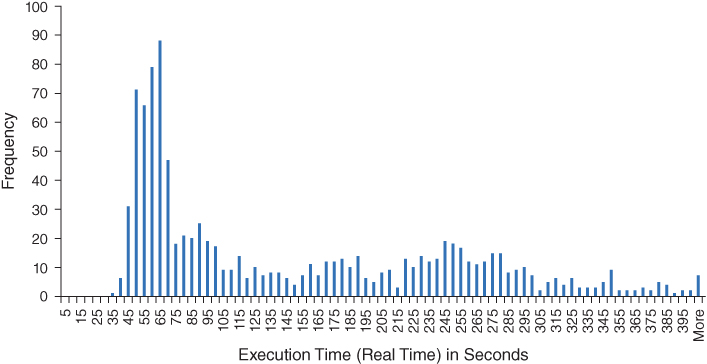
Figure 7.6 Histogram of Real Time for Sorting 10 Million Observations
As Figure 7.6 demonstrates, real time measurements are anything but normalized—in fact, the graph represents the typical platykurtic, right-skewed distribution of real time measurements. Because real time is influenced by external factors such as other SAS programs, additional software, or system administrative activities such as virus scanning, it can be incredibly unpredictable. For example, the SORT procedure took a minimum and maximum of 34.9 and 560.4 seconds, respectively, with a mean of 145.0 seconds and standard deviation of 100.1 seconds! While some of this variability can be eliminated by reducing external processes that are running in the SAS environment, this reduction likely would not represent the typical operational environment.
A more consistent method of calculating performance speed is to utilize CPU time, which is demonstrated in the SAS log when the NOFULLSTIMER option is selected, or which can be calculated by adding user CPU time and system CPU time when the FULLSTIMER option is selected. Figure 7.7 demonstrates the real time measurements (from Figure 7.6) overlaid with CPU time measurements for the same 1,000 iterations of the SORT procedure.
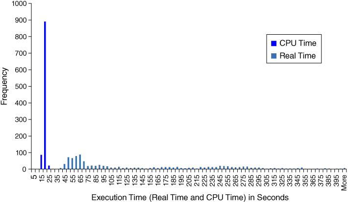
Figure 7.7 Histogram of Real Time and CPU Time for Sorting 10 Million Observations
Figure 7.7 puts in perspective the tremendous variation in real time as compared with CPU time. CPU time tends to be very consistent, demonstrating a highly leptokurtic but only slightly right-skewed distribution. For example, the CPU time for the SORT procedure took a minimum and maximum of 13.1 and 27.3 seconds, respectively, with a mean of 16.8 seconds and standard deviation of only 1.5 seconds. The total amount of CPU time—irrespective of its distribution—will also be less than real time because factors such as external processes and the basic I/O functionality required to write the sorted data set incur additional real time. One exception to this rule exists: multithreaded processes can incur a greater CPU time than run time because all parallel threads incur CPU time while real time only measures from the start of the first thread to the completion of the last.
Real time and CPU time each have their respective uses. Customers and most stakeholders will be concerned only with real time because it measures a real construct—how long software took to complete. For this reason, real time is exclusively included within requirements documentation, SLAs, performance logs, and failure logs. For example, if analytic software took 20 minutes too long to complete, stakeholders will not care about its lower CPU time—only the unacceptable real time. During development, optimization, and testing, however, CPU time is invaluable in comparing technical methodologies because it eliminates the variability inherent in real time metrics. In other words, you can run a SAS process a few times and have a decent idea of whether it decreases or increases performance as compared with another method. Once methods have been compared using CPU time, however, testing and validation must ultimately demonstrate that real time—not CPU time—meets established needs and requirements and that its variability will not result in performance failures during software operation. Real time and CPU time are further discussed in the “CPU Processing” section in chapter 8, “Efficiency.”
Inefficiency Elbow
The inefficiency elbow is a phenomenon that occurs when software fails to scale to increased data volume, typically causing slowed performance and later functional failure. The SORT procedure most notably displays the inefficiency elbow, which occurs when RAM is exhausted and SAS switches to using less efficient virtual memory. Other SAS processes may hit a wall—at which point they suddenly fail with an out-of-memory error—instead of an elbow. The telltale sequela of the inefficiency elbow is substantially decreased software speed; however, because the cause is rooted squarely in the failure of system resource utilization to scale as data volume increases, this topic is described and demonstrated in the “Memory” section in chapter 8, “Efficiency,” and in the “Inefficiency Elbow” section in chapter 9, “Scalability.”
WHAT'S NEXT?
This chapter has thrown caution to the wind, touting the need for software to go as fast as possible without questioning the utilization (or monopolization) of system resources. As the “Parallel Processing” section demonstrates, however, speed isn't free—it incurs higher memory and CPU consumption, and often makes software less efficient. In chapter 8, “Efficiency,” the real costs of performance are revealed, as system resources—including CPU usage, memory usage, I/O processing, and disk space—are explored.