
CHAPTER 17
ADJUSTMENT OF GNSS NETWORKS
17.1 INTRODUCTION
For the past seven decades, NASA and the US military have been engaged in a space research program to develop a precise positioning and navigation system. The first-generation system, called TRANSIT, used six satellites and was based on the doppler principle. TRANSIT was made available for commercial use in 1967, and shortly thereafter its use in surveying began. The establishment of a worldwide network of control stations was among its earliest and most valuable applications. Point positioning using TRANSIT required very lengthy observing sessions, and its accuracy was at the 1 m level. Thus, in surveying it was suitable only for control work on networks consisting of widely spaced points. It was not satisfactory for everyday surveying applications such as traversing or engineering layout.
Encouraged by the success of TRANSIT, a new research program was developed that ultimately led to the creation of the Navigation Satellite Tracking and Ranging (NAVSTAR) Global Positioning System (GPS). This second-generation positioning and navigation system utilizes a nominal constellation of 24 orbiting satellites. The accuracy of GPS was a substantial improvement over that of the TRANSIT system, and the disadvantage of lengthy observing sessions was also eliminated. Although developed for military applications, civilians, including surveyors, also found uses for the GPS system.
Since its introduction, GPS has been used extensively. It has been found to be reliable, efficient, and capable of yielding extremely high accuracies. GPS observations can be taken day or night and in any weather conditions. A significant advantage of GPS is that visibility between surveyed points is not necessary. Thus, the time-consuming process of clearing lines of sight is avoided. Although most of the early applications of GPS were in control work, improvements have now made the system convenient and practical for use in virtually every type of survey including property surveys, topographic mapping, and construction staking.
Today, several countries have or are in the process of developing satellite positioning systems similar to GPS. These combined systems are now known as global navigation satellite systems (GNSSs). In keeping with these changes, this book has adopted GNSS in reference to all of these satellite-positioning systems.
This chapter provides a brief introduction to GNSS surveying. We explain the basic observations involved in the system, discuss errors in those observations, describe the nature of the adjustments needed to account for those errors, and give the procedures for making adjustments of networks surveyed using GNSS. An example problem is given to demonstrate the procedures.
17.2 GNSS OBSERVATIONS
![]() Fundamentally, global navigation satellite systems operate by observing distances from receivers located on ground stations of unknown locations to orbiting GNSS satellites whose positions are precisely known. Thus, conceptually, GNSS surveying is similar to conventional resection, in that distances are observed with an EDM instrument from an unknown station to several control points. (The conventional resection procedure was discussed in Chapter 15 and illustrated in Example 15.2.) Of course, there are some major differences between GNSS position determination and conventional resection. Among them is the process of observing distances and the fact that the control stations used in GNSS work are satellites, which removes the need for intervisibility between stations.
Fundamentally, global navigation satellite systems operate by observing distances from receivers located on ground stations of unknown locations to orbiting GNSS satellites whose positions are precisely known. Thus, conceptually, GNSS surveying is similar to conventional resection, in that distances are observed with an EDM instrument from an unknown station to several control points. (The conventional resection procedure was discussed in Chapter 15 and illustrated in Example 15.2.) Of course, there are some major differences between GNSS position determination and conventional resection. Among them is the process of observing distances and the fact that the control stations used in GNSS work are satellites, which removes the need for intervisibility between stations.
Distances are determined in GNSS surveying by taking observations on these transmitted satellite signals. Two different observational procedures are used: positioning by pseudoranging, and positioning by carrier phase-shift observations. Pseudoranging involves determining distances (ranges) between satellites and receivers by observing precisely the time it takes transmitted signals to travel from satellites to ground receivers. With the velocity and travel times of the signals known, the pseudoranges can be computed. Finally, based on these ranges, the positions of the ground stations can be calculated. Because pseudoranging is based on observing pseudorandom noise (PRN) codes, this GPS observation technique is also often referred to as the code measurement procedure.
In the carrier phase-shift procedure, the quantities observed are phase changes that occur as a result of the carrier wave traveling from the satellites to the receivers. The principle is similar to the phase-shift method employed by electronic distance-measuring instruments. However, a major difference is that the satellites are moving, and the signals are not returned to the transmitters for “true” phase-shift measurements. Instead, the phase shifts must be observed at the receivers. But to make true phase-shift observations, the clocks in the satellites and receivers would have to be perfectly synchronized, which, of course, cannot be achieved. To overcome this timing problem and to eliminate other errors in the system, differencing techniques (taking differences between phase observations) are used. Various differencing procedures can be applied. Single differencing is achieved by simultaneously observing two satellites with one receiver. Single differencing eliminates satellite clock biases. Double differencing (subtracting the results of single differences from two receivers) eliminates receiver clock biases and other systematic errors.
Another problem in making carrier-phase observations is that only the phase shift of the last cycle of the carrier wave is observed, and the number of full cycles in the travel distance is unknown. (Recall in EDM work that this problem was overcome by transmitting longer wavelengths and observing their phase shifts.) Again, because the satellites are moving, this cannot be done in GNSS work. However, by extending the differencing technique to what is called triple differencing, this ambiguity in the number of cycles cancels out of the solution. Triple differencing consists of differencing the results of two double differences, and thus involves making observations at two different times to two satellites from two stations.
Rather than performing triple differencing, a more common technique used in today's software to determine ambiguities is to develop probable ranges for each of the range ambiguities. These ranges are analyzed using differing combinations from least squares adjustments. The final objective being the determination of the most probable combination of ranges that provides the most probable solution for the position of the receiver.
In practice, when surveys are done by observing carrier phases, four or more satellites are observed simultaneously using two or more receivers located on ground stations. Also, the observations are repeated many times. This produces a very large number of redundant observations, from which many difference combinations can be computed.
Of the two GNSS observing procedures, pseudoranging yields a somewhat lower order of accuracy, but it is preferred for navigation use because it gives instantaneous point positions of satisfactory accuracy. The carrier-phase technique produces a higher order of accuracy and is therefore the choice for high-precision surveying applications. Adjustment of carrier-phase GNSS observations is the subject of this chapter.
The differencing techniques used in carrier-phase observations, described briefly above, do not yield positions directly for the points occupied by receivers. Rather, baselines (vector distances between stations) are determined. These baselines are computed in terms of their coordinate difference components ΔX, ΔY, and ΔZ. These coordinate differences are reported in the reference three-dimensional rectangular coordinate system described in Section 17.4.
To use the GNSS carrier-phase procedure in surveying, at least two receivers located on separate stations must be operated simultaneously. For example, assume that two stations A and B were occupied for an observing session, that station A is a control point, and that station B is a point of unknown position. The session would yield coordinate differences ΔXAB, ΔYAB, and ΔZAB between stations A and B. The X, Y, Z coordinates of station B can then be obtained by adding the baseline components to the coordinates of A, as

Because carrier-phase observations do not yield point positions directly, but rather give baseline components, this method of GNSS surveying is referred to as relative positioning. In practice, often more than two receivers are used simultaneously in relative positioning, which enables more than one baseline to be determined during each observing session. Also, after the first observing session, additional points are interconnected in the survey by moving the receivers to other nearby stations. In this procedure, at least one receiver is left on one of the previously occupied stations. By employing this technique, a network of interconnected points can be created. Figure 17.1 illustrates an example of a GNSS network. In this figure, stations A and B are control stations, and stations C, D, E, and F are points of unknown positions. Creation of such networks is a common procedure employed in GPS relative positioning work.

FIGURE 17.1 GPS survey network.
17.3 GNSS ERRORS AND THE NEED FOR ADJUSTMENT
As in all types of surveying observations, GNSS observations contain errors. The principal sources of these errors are (1) orbital errors in the satellite, (2) signal transmission timing errors due to atmospheric conditions, (3) receiver errors, (4) multipath errors (signals being reflected so that they travel indirect routes from satellite to receiver), and (5) miscentering errors of the receiver antenna over the ground station, and in height measuring errors above the station. To account for these and other errors, and to increase the precisions of point position, GNSS observations are very carefully made according to strict specifications, and redundant observations are taken. The fact that errors are present in the observations makes it necessary to analyze the observations for acceptance or rejection. Also, because redundant observations have been made, they must be adjusted so that all observed values are consistent.
In GNSS surveying work where the observations are made using carrier phases, there are two stages where least squares adjustment is applied typically. The first is in processing the redundant carrier phase-shift observations to obtain the adjusted baseline components (ΔX, ΔY, ΔZ), and the second is in adjusting networks of stations wherein the baseline components have been observed. The latter adjustment is discussed in more detail later in the chapter.
17.4 REFERENCE COORDINATE SYSTEMS FOR GNSS OBSERVATIONS
In GNSS surveys, three different reference coordinate systems are involved. First, the satellite positions at the instants of their observation are given in a space-related Xs, Ys, Zs three-dimensional rectangular coordinate system. This coordinate system is illustrated in Figure 17.2. In the figure, the elliptical orbit of a satellite is shown. It has one of its two foci at G, the Earth's center of gravity. Two points, perigee (point where the satellite is closest to G) and apogee (point where the satellite is farthest from G), define the line of apsides. This line, which also passes through the two foci, is the Xs axis of the satellite reference coordinate system. The origin of the system is at G, the Ys axis is in the mean orbital plane, and Zs is perpendicular to the Xs−Ys plane. Since the instantaneous position of the satellites is used in computations, values of Zs are assumed to be zero. For each specific instant of time that a given satellite is observed, its coordinates are calculated in its unique Xs, Ys, Zs system.

FIGURE 17.2 Satellite reference coordinate system.
In processing GNSS observations, all Xs, Ys, Zs coordinates that were computed for satellite observations are converted to a common Earth-related Xe, Ye, Ze three-dimensional geocentric coordinate system. This Earth-centered, Earth-fixed coordinate system, illustrated in Figure 17.3, is also commonly called the terrestrial geocentric coordinate system, or simply the geocentric system. It is in this system that the baseline components are computed based on the differencing of observed carrier-phase observations. The origin of this coordinate system is at the Earth's gravitational center. The Ze axis coincides with the Earth's Conventional Terrestrial Pole (CTP) axis, the Xe–Ye plane is perpendicular to the Ze axis, and the Xe axis passes through the Greenwich Meridian. To convert coordinates from the space related (Xs, Ys, Zs) system to the Earth-centered, Earth-related (Xe, Ye, Ze) geocentric system, six parameters are needed. These are (a) the inclination angle i (the angle between the orbital plane and the Earth's equatorial plane); (b) the argument of perigee ω (the angle observed in the orbital plane between the equator and the line of apsides); (c) right ascension of the ascending node Ω (the angle observed in the plane of the Earth's equator from the vernal equinox to the line of intersection between the orbital and equatorial planes); (d) the Greenwich hour angle of the vernal equinox γ (the angle observed in the equatorial plane from the Greenwich meridian to the vernal equinox); (e) the semimajor axis of the orbital ellipse, a; and (f) the eccentricity, e, of the orbital ellipse. The first four parameters are illustrated in Figure 17.3. For any satellite at any instant of time, these four parameters are available. Software provided by GNSS equipment manufacturers computes the Xs, Ys, Zs coordinates of satellites at the instance of observation and transforms these coordinates into the Xe, Ye, Ze geocentric coordinate system used for computing the baseline components.

FIGURE 17.3 Earth-related, three-dimensional coordinate system used in GPS carrier-phase differencing computations.
In order for the results of the baseline computations to be useful to local surveyors, the Xe, Ye, Ze coordinates must be converted to geodetic coordinates of latitude, longitude, and height. The geodetic coordinate system is illustrated in Figure 17.4, where the parameters are symbolized by φ, λ, and h, respectively. Geodetic coordinates are referenced to the World Geodetic System of 1984, which employs the WGS84 ellipsoid and is defined by the ground coordinates of the tracking stations. The center of this ellipsoid is oriented at the Earth's gravitational center. Its origin varies from the origin of the NAD 83 datum by 1.5 m. The differences between the two reference frames will be discussed in Chapter 24. From latitude and longitude, state plane coordinates, which are more convenient for use by local surveyors, can be computed.

FIGURE 17.4 Geodetic coordinates (with the Earth-centered, Earth-fixed coordinates XP, YP, and ZP geocentric coordinate system superimposed).
It is important to note that geodetic heights are not orthometric heights (elevations referred to the geoid). To convert geodetic heights to orthometric heights, the geoid heights (vertical distances between the ellipsoid and geoid) must be subtracted from geodetic heights. That is,
where h is the geodetic height of the point, H is the orthometric height (elevation) of the point, and N is the geoid height (separation between the geoid and ellipsoid) below the point.
17.5 CONVERTING BETWEEN THE TERRESTRIAL AND GEODETIC COORDINATE SYSTEMS
GNSS networks must include at least one control point, but more are preferable. The geodetic coordinates of these control points will normally be given from a previous GNSS survey or Continuously Operating Reference Stations (CORSs). Prior to processing carrier-phase observations to obtain adjusted baselines for a network, the coordinates of the control stations in the network must be converted from their geodetic values into the Earth-centered, Earth-related Xe, Ye, Ze geocentric system. The equations for making these conversions are
In the equations above, h is the geodetic height of the point; φ the geodetic latitude of the point; and λ the geodetic longitude of the point. Also, e is eccentricity for the ellipsoid, which is computed as
or

where f is the flattening factor of the ellipsoid; a and b are the semimajor and semiminor axes, respectively, of the ellipsoid;1 and N is the normal to the ellipsoid at the point, which is computed from

Note that the normal at a point, N, in Equations (17.2) through (17.6) should not be confused with the geoid height mentioned previously.
17.6 APPLICATION OF LEAST SQUARES IN PROCESSING GNSS DATA
As stated previously, a least squares adjustment is used at two different stages in processing GNSS carrier phase-shift observations. First, it is applied in the adjustment that yields baseline components between stations from the redundant carrier phase observations. Recall that in this procedure, differencing techniques are employed to compensate for errors in the system and to resolve the cycle ambiguities. In the solution, observation equations are written that contain the differences in coordinates between stations as parameters. The reference coordinate system for this adjustment is the Xe, Ye, Ze geocentric system. A highly redundant system of equations is obtained because, as described earlier, a minimum of four (and often more) satellites are simultaneously tracked using at least two (and often more) receivers. Furthermore, many repeat observations are taken. This system of equations is solved by least squares to obtain the most probable ΔX, ΔY, ΔZ components of the baseline vectors. The development of these observation equations is beyond the scope of this book, and thus their solution by least squares is also not covered herein.3
Software furnished by manufacturers of GNSS receivers will process observed phase changes to form the differencing observation equations, perform the least squares adjustment, and output the adjusted baseline vector components. The software will also output the covariance matrix, which expresses the correlation between the ΔX, ΔY, ΔZ components of each baseline. The software is proprietary and thus cannot be included herein.
The second stage where least-squares adjustments are employed in processing GNSS observations is in adjusting baseline vector components in networks. This adjustment is made after the least squares adjustment of the carrier–phase observations is completed. It is also done in the Xe, Ye, Ze geocentric coordinate system. In network adjustments, the goal is to make all X coordinates (and all X-coordinate differences) consistent throughout the figure. The same objective applies for all Y coordinates and for all Z coordinates. As an example, consider the GPS network shown in Figure 17.1. It consists of two control stations and four stations whose coordinates are to be determined. A summary of the baseline observations obtained from the least squares adjustment of carrier phase-shift observations for this figure is given in Table 17.1. The covariance matrix elements that are listed also in Table 17.1 are used for weighting the observations. These will be discussed in Section 17.8, and for the moment they can be ignored.
TABLE 17.1 Observed Baseline Data for the Network of Figure17.1
| (1) | (2) | (3) | (4) | (5) | (6) | (7) | (8) | (9) | (10) | (11) |
| From | To | ΔX | ΔY | ΔZ | Covariance Matrix Elements | |||||
| A | C | 11,644.2232 | 3,601.2165 | 3,399.2550 | 9.884E−4 | −9.580E−6 | 9.520E−6 | 9.377E−4 | −9.520E−6 | 9.827E−4 |
| A | E | −5,321.7164 | 3,634.0754 | 3,173.6652 | 2.158E−4 | −2.100E−6 | 2.160E−6 | 1.919E−4 | −2.100E−6 | 2.005E−4 |
| B | C | 3,960.5442 | −6,681.2467 | −7,279.0148 | 2.305E−4 | −2.230E−6 | 2.070E−6 | 2.546E−4 | −2.230E−6 | 2.252E−4 |
| B | D | −11,167.6076 | −394.5204 | −907.9593 | 2.700E−4 | −2.750E−6 | 2.850E−6 | 2.721E−4 | −2.720E−6 | 2.670E−4 |
| D | C | 15,128.1647 | −6,286.7054 | −6,371.0583 | 1.461E−4 | −1.430E−6 | 1.340E−6 | 1.614E−4 | −1.440E−6 | 1.308E−4 |
| D | E | −1,837.7459 | −6,253.8534 | −6,596.6697 | 1.231E−4 | −1.190E−6 | 1.220E−6 | 1.277E−4 | −1.210E−6 | 1.283E−4 |
| F | A | −1,116.4523 | −4,596.1610 | −4,355.9062 | 7.475E−5 | −7.900E−7 | 8.800E−7 | 6.593E−5 | −8.100E−7 | 7.616E−5 |
| F | C | 10,527.7852 | −994.9377 | −956.6246 | 2.567E−4 | −2.250E−6 | 2.400E−6 | 2.163E−4 | −2.270E−6 | 2.397E−4 |
| F | E | −6,438.1364 | −962.0694 | −1,182.2305 | 9.442E−5 | −9.200E−7 | 1.040E−6 | 9.959E−5 | −8.900E−7 | 8.826E−5 |
| F | D | −4,600.3787 | 5,291.7785 | 5,414.4311 | 9.330E−5 | −9.900E−7 | 9.000E−7 | 9.875E−5 | −9.900E−7 | 1.204E−4 |
| F | B | 6,567.2311 | 5,686.2926 | 6,322.3917 | 6.643E−5 | −6.500E−7 | 6.900E−7 | 7.465E−5 | −6.400E−7 | 6.048E−5 |
| B | F | −6,567.2310 | −5,686.3033 | −6,322.3807 | 5.512E−5 | −6.300E−7 | 6.100E−7 | 7.472E−5 | −6.300E−7 | 6.629E−5 |
| A | F | 1,116.4577 | 4,596.1553 | 4,355.9141 | 6.619E−5 | −8.000E−7 | 9.000E−7 | 8.108E−5 | −8.200E−7 | 9.376E−5 |
| Aa | B | 7,683.6883 | 10,282.4550 | 10,678.3008 | 7.2397E−4 | −7.280E−6 | 7.520E−6 | 6.762E−4 | −7.290E−6 | 7.310E−4 |
a Fixed baseline used only for checking, but not included in adjustment.
A network adjustment of Figure 17.1 should yield adjusted X coordinates for the stations (and adjusted coordinate differences between stations) that are all mutually consistent. Specifically for this network, the adjusted X coordinate of station C should be obtained by adding ΔXAC to the X coordinate of station A; and the same value should be obtained by adding ΔXBC to the X coordinate of station B, or by adding ΔXDC to the X coordinate of station D, and so on. Equivalent conditions exist for the Y and Z coordinates. Note that these conditions do not exist for the data of Table 17.1, which contains the unadjusted baseline observations. The procedure of adjusting GNSS networks is described in detail in Section 17.8, and an example is given.
17.7 NETWORK PREADJUSTMENT DATA ANALYSIS
Prior to adjusting GNSS networks, a series of procedures should be followed to analyze the data for internal consistency and to eliminate possible blunders. No control points are needed for these analyses. Depending on the actual observations taken and the network geometry, these procedures may consist of analyzing (1) differences between fixed and observed baseline components, (2) differences between repeated observations of the same baseline components, and (3) loop closures. After making these analyses, a minimally constrained adjustment is usually performed that will help isolate any blunders that may have escaped the first set of analyses. Procedures for making these analyses are described in the following subsections.
17.7.1 Analysis of Fixed Baseline Measurements
GNSS job specifications often require that baseline observations be taken between fixed control stations. The benefit of making these observations is to verify the accuracy of both the GNSS observational system and the control being held fixed. Obviously, smaller the discrepancies between observed and known baseline lengths mean more accurate observations. If the discrepancies are too large to be tolerated, the conditions causing them must be investigated before proceeding further. Note that in the data of Table 17.1, one fixed baseline (between control points A and B) was observed. Table 17.2 gives the data for comparing the observed and fixed baseline components. The observed values are listed in column (2), and the fixed components are given in column (3). To compute the fixed values, Xe, Ye, Ze geocentric coordinates of the two control stations are first determined from their geodetic coordinates according to procedures discussed in Section 17.5. Then the ΔX, ΔY, ΔZ differences between the Xe, Ye, Ze coordinates for the two control stations are determined. Differences (in meters) between the observed and fixed baseline components are given in column (4). Finally the differences, expressed in parts per million (ppm), are listed in column (5). These ppm values are obtained by dividing column (4) differences by their corresponding total baseline lengths and multiplying by 1,000,000. A determination of the acceptability of the computed ppm can be evaluated based on published standards such as the Federal Geodetic Control Subcommittee's Geometric Geodetic Accuracy Standards and Specifications for Using GPS Relative Positioning Techniques.
TABLE 17.2 Comparisons of Observed and Fixed Baseline Components
| (1) | (2) | (3) | (4) | (5) |
| Component | Observed (m) | Fixed (m) | Difference (m) | PPMa |
| ΔX | 7,683.6883 | 7,683.6809 | 0.0074 | 0.44 |
| ΔY | 10,282.4550 | 10,282.4537 | 0.0013 | 0.08 |
| ΔZ | 10,678.3008 | 10,678.3058 | 0.0050 | 0.30 |
a The total baseline length used in computing these ppm values was 16,697 m, which was derived from the square root of the sum of the squares of ΔX, ΔY, and ΔZ values.
When the standards are inappropriate for the survey method being performed, the baselines can also be compared against the estimated error in the line based on manufacturer's specifications for the particular survey method used. Since each receiver in a baseline adds in an additional three-dimensional setup error σs, the error in any observed baseline can be estimated as
where a is the specified constant error for an observed baseline and L is the length of the baseline observed. For example, the typical specified accuracy for a baseline determined using static surveying procedures is 5 mm + 1 ppm, where a is 5 mm and 1 the ppm. Baseline AB is approximately 16,697 m in length. Based on the previously stated accuracies and assuming setup errors of 0.0015 m for each receiver. Using Equation (17.13), the estimated error in the baseline is

Since the baseline is determined from more than 30 individual epochs of data with multiple satellite observations typically, the normal distribution multiplier can be used to raise this uncertainty to an appropriate percent probability. For example, at 95% the estimated error in the baseline could be as much as 1.96(0.0176), which equals ±0.034 m. Since the actual misclosure between the observed and fixed baseline is only ![]() , it is well within the 95% range of the estimated misclosure.
, it is well within the 95% range of the estimated misclosure.
17.7.2 Analysis of Repeat Baseline
Another procedure employed in evaluating the consistency of the observed data and in weeding out blunders is to make repeat observations of certain baselines. These repeat observations are taken in different sessions and the results compared. The repeat baselines provide checks on field and office procedures and aid in isolating poor practices. For example, in the data of Table 17.1, baselines AF and BF were repeated. Table 17.3 gives comparisons of these observations using the same procedure that was used in Table 17.2. Again, the ppm values listed in column (5) use the total baseline lengths in the denominator, which are computed from the square root of the sum of the squares of the measured baseline components. It is wise to perform repeat observations at the end of each day to check the repeatability of the software, hardware, and field procedures.
TABLE 17.3 Comparisons of Repeat Baseline Measurements
| Component | First Observation | Second Observation | Difference (m) | PPM |
| ΔXAF | 1116.4577 | −1116.4523 | 0.0054 | 0.84 |
| ΔYAF | 4596.1553 | −4596.1610 | 0.0057 | 0.88 |
| ΔZAF | 4355.9141 | −4355.9062 | 0.0079 | 1.23 |
| ΔXBF | −6567.2310 | 6567.2311 | 0.0001 | 0.01 |
| ΔYBF | −5686.3033 | 5686.2926 | 0.0107 | 1.00 |
| ΔZBF | −6322.3807 | 6322.3917 | 0.0110 | 1.02 |
The Federal Geodetic Control Subcommittee (FGCS) has developed a document titled “Geometric Geodetic Accuracy Standards and Specifications for Using GPS Relative Positioning Techniques.” It is intended to serve as a guideline for planning, executing, and classifying geodetic surveys performed by GNSS relative positioning methods. This document may be consulted to determine whether or not the ppm values of column (5) are acceptable for the required order of accuracy for the survey. Besides ppm requirements, the FGCS guidelines specify other criteria that must be met for the different orders of accuracy in connection with repeat baseline observations. Again the acceptability of the line can be computed based on the FGCS guidelines or by comparing the baseline against the manufacturer's specified accuracies.
Developing a statistical test for repeat baselines may be impossible since, it must be remembered that we are comparing the difference between two observations. The proper statistical test is demonstrated in Section 18.18. However, this test requires the knowledge about each baselines computed error, the number of redundant observations, and the total number of observations. While the root-mean-square (RMS) error is typically reported by software, the number of redundant and total observations is seldom provided in a baseline adjustment report. Thus, another approach needs to be considered. One method might simply be to see if the linear difference between the two baseline observations is greater than the estimated error for a baseline of this length. In this case, Equation (17.13) will yield the estimated error in the length of the line, which can be multiplied to an appropriate level of probability. Then, similar to the procedures used for fixed baseline observations, the actual error can be compared against the estimated value. Although this procedure lacks the rigor of a proper statistical test, it should provide enough information to isolate baseline observations that have obvious problems. This method is demonstrated in Example 17.3 with repeat baselines FA and AF.
17.7.3 Analysis of Loop Closures
GNSS networks will typically consist of many interconnected closed loops. For example, in the network of Figure 17.1, a closed loop is formed by points ACBDEA. Similarly, ACFA, CFBC, BDFB, and so on, are other closed loops. For each closed loop, the algebraic sum of the ΔX components should equal zero. The same condition should exist for the ΔY and ΔZ components. These loop misclosure conditions are very similar to the leveling loop misclosures imposed in differential leveling and latitude and departure misclosures imposed in closed-polygon traverses. An unusually large misclosure within any loop will indicate that either a blunder or a large random error exists in one (or more) of the baselines of the loop.
To compute loop misclosures, the baseline components are added algebraically for the chosen loop. For example, the misclosure in X components for loop ACBDEA would be computed as
where cx is the loop misclosure in X coordinates. Similar equations apply for computing misclosures in Y and Z coordinates.
Substituting numerical values into Equation (17.14), the misclosure in X coordinates for loop ACBDEA is

Similarly, misclosures in Y and Z coordinates for that loop are
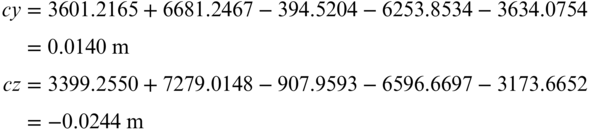
For evaluation purposes, loop misclosures are expressed in terms of the ratios of resultant misclosures to the total loop lengths. They are given in ppm. For any loop, the resultant misclosure is the square root of the sum of the squares of its cx, cy, and cz values and for loop ACBDEA the resultant is 0.0505 m. The total length of a loop is computed by summing its legs, each leg being computed from the square root of the sum of the squares of its observed ΔX, ΔY, and ΔZ values. For loop ACBDEA, the total loop length is 50,967 m, and the misclosure ppm ratio is therefore (0.0505/50,967)(1,000,000) = 0.99 ppm. Again, these ppm ratios can be compared against values given in the FGCS guidelines to determine if they are acceptable for the order of accuracy of the survey. As was the case with repeat baseline observations, the FGCS guidelines also specify other criteria that must be met in loop analyses besides the ppm values.
These misclosures can also be checked against manufacturer specifications. In this case, Equation (17.13) can be modified as
where n is the number of baselines in the loop, L is the overall length of the loop, and the other terms are as defined in Equation (17.13).
Assuming as before an accuracy of 5 mm + 1 ppm and setup errors of 0.0015 m, the estimated error in the loop is

Again, the actual misclosure is within the estimated error of the baseline at a 68% probability. As with Equation (17.13), multipliers derived from the normal distribution can be used to estimate errors at any other level of probability.
For any network, enough loop closures should be computed so that every baseline is included within at least one loop. This should expose any large blunders that exist. If a blunder does exist, its location can be determined through additional loop–closure analyses often. For example, assume that the misclosure of loop ACDEA discloses the presence of a blunder. By also computing the misclosures of loops AFCA, CFDC, DFED, and EFAE, the baseline containing the blunder can often be detected. In this example, if a large misclosure was found in loop DFED and all other loops appeared to be blunder free, the blunder could be in line DE.
A computer program included within the software package ADJUST can determine these loop–closure computations. Figure 17.5 shows the resultant loop misclosures. The “LC” column lists the actual misclosure of each loop. The “s” column list the estimated error in the loop based on user-supplied setup errors, and estimated errors in the observed GPS baseline vectors. This column is at 68% and must be multiplied by the appropriate multiplier to raise it to another level of probability. Finally, the “ppm” column lists the computed parts-per-million error for each loop. The help file that accompanies the software explains the format of the data file shown in Figure 17.6. This file lists the number of baseline vectors (14) followed by the each baseline vector with a consecutive number. These numbers are used to determine which baseline vectors are included in any loop. This particular file lists the six loops discussed previously. For example, loop ACBDEA is defined as “1 3 4 6 2” where “1” is baseline AC, “3” is BC, and so on. As can be seen with baseline EA, the software will automatically reverse the signs of the baseline vector components when the letters are shown in the reverse order.

FIGURE 17.5 Results of loop misclosure computations for example in Section 17.7.3.

FIGURE 17.6 ADJUST data file for computing loop misclosure as discussed in Section 17.7.3.
17.7.4 Minimally Constrained Adjustment
Prior to making the final adjustment of baseline observations in a network, a “minimally constrained” least squares adjustment is usually performed. In this adjustment, sometimes called a “free” adjustment, any station in the network may be held fixed with arbitrary coordinates. All other stations in the network are therefore free to adjust as necessary to accommodate the baseline observations and network geometry. The residuals that result from this adjustment are strictly related to the baseline observations and not to faulty control coordinates. These residuals are examined and, from them, blunders that may have gone undetected through the first set of analyses can be found and eliminated. Often these adjustments use statistical blunder detection methods discussed in Chapter 21.
17.8 LEAST SQUARES ADJUSTMENT OF GNSS NETWORKS
![]() As noted earlier, because GNSS networks contain redundant observations, they must be adjusted to make all coordinate differences consistent. In applying least squares to the problem of adjusting baselines in GNSS networks, observation equations are written that relate station coordinates to the observed coordinate differences and their residual errors. To illustrate this procedure, consider the example of Figure 17.1. For line AC of this figure, an observation equation can be written for each observed baseline component as
As noted earlier, because GNSS networks contain redundant observations, they must be adjusted to make all coordinate differences consistent. In applying least squares to the problem of adjusting baselines in GNSS networks, observation equations are written that relate station coordinates to the observed coordinate differences and their residual errors. To illustrate this procedure, consider the example of Figure 17.1. For line AC of this figure, an observation equation can be written for each observed baseline component as

Similarly the observation equations for the baseline components of line CD are

Observation equations of the form above are written for all observed baselines in any figure. For Figure 17.1 there were a total of 13 observed baselines, so the number of observation equations that can be developed is 39. Also each of stations C, D, E, and F has three unknown coordinates, for a total of 12 unknowns in the problem. Thus, there are 39 − 12 = 27 redundant observations in the network. The 39 observation equations can be expressed in matrix form as
If the observation equations for adjusting the network of Figure 17.1 are written in the same order that the observations are listed in Table 17.1, the A, X, L, and V matrices are

The numerical values of the elements of the L matrix are determined by rearranging the observation equations. Its first three elements are for the ΔX, ΔY, ΔZ baseline components of line AC, respectively. Those elements are calculated as follows

The other elements of the L matrix are formed in the same manner as demonstrated for baseline AC. However before numerical values for the L matrix elements can be obtained, the Xe, Ye, Ze geocentric coordinates of all control points in the network must be computed. This is done by following the procedures described in Section 17.5 and demonstrated by Example 17.1. That example problem provided the Xe, Ye, Ze coordinates of control points A and B of Figure 17.1, which are used to compute the elements of the L matrix given above.
Note that the observation equations for GNSS network adjustment are linear and that the only nonzero elements of the A matrix are either 1 or −1. This is the same type of matrix that was developed in adjusting differential leveling networks by least squares. In fact, GNSS network adjustments are performed in the very same manner, with the exception of the stochastic model. In relative positioning, the three observed baseline components are correlated. Therefore, a covariance matrix of dimensions 3 × 3 is derived for each baseline as a product of the least squares adjustment of the carrier phase observations. This covariance matrix is used to weight the observations in the network adjustment in accordance with Equation (10.4). The weight matrix for any GNSS network is therefore a block-diagonal type, with an individual 3 × 3 matrix for each observed baseline on the diagonal. When more than two receivers are used, additional 3 × 3 matrices are created in the off-diagonal region of the matrix to provide the correlation that exists between the simultaneously observed baselines. All other elements of the matrix are zeros. Since commercial software computes individual baseline vectors, the correlation (off-diagonal 3 × 3 matrices) between simultaneously observed baseline vectors using three or more receivers is not determined. This fact results in a stochastic model that is incorrect theoretically and can cause problems in post-adjustment statistical analysis.
The covariances for the observations in Table 17.1 are given in columns (6) through (11). Only the six lower-triangular elements of the 3 × 3 covariance matrix for each observation are listed. However, because the covariance matrix is symmetrical, this gives complete weighting information. Columns 6 through 11 list ![]() , respectively. Thus, the full 3 × 3 covariance matrix for baseline AC is
, respectively. Thus, the full 3 × 3 covariance matrix for baseline AC is

The complete weight matrix for the example network of Figure 17.1 has dimensions of 39 × 39. After inverting the full matrix and multiplying by the a priori estimate for the reference variance, ![]() , in accordance with Equation (10.4), the weight matrix for the network of Figure 17.1 is as follows. (Note that
, in accordance with Equation (10.4), the weight matrix for the network of Figure 17.1 is as follows. (Note that ![]() is taken as 1.0 for this computation, and that no correlation between separate baselines is included.)
is taken as 1.0 for this computation, and that no correlation between separate baselines is included.)


FIGURE 17.7 ADJUST data file for the example in Section 17.8.
The system of observation Equations (17.8) is solved by least squares using Equation (11.35). This yields the most probable values for the coordinates of the unknown stations. The ADJUST data file is shown in Figure 17.7. As with other ADJUST data files, the first line is a description of the contents of the file. This line is followed with the number of control stations, number of unknown stations, and number of baseline vectors. The control stations are listed with a point identifier that cannot contain a space, comma, or tab since these characters are used as entry delimiters. The point identifier is followed by the point's geocentric coordinates in the order of X, Y, and Z. Following the control station entries is a listing of each baseline vector. These lines have the format of the primary station identifier, secondary station identifier, baseline vector components of ΔX, ΔY, and ΔZ. The baseline vector components are followed by the covariance elements for the vector given in the same order as listed in Table 17.1. The ADJUST data file Example from Section 17-8.dat is available on the companion website for this book. For those wishing to program in a higher-level language, the Mathcad® worksheet C17.xmcd is available on the companion website. A listing of the adjustment of the data in Figure 17.1 obtained using the program ADJUST follows.
Control stationsStation X Y Z==================================================================================A 402.35087 -4652995.30109 4349760.77753B 8086.03178 -4642712.84739 4360439.08326Distance VectorsFrom To ΔX ΔY ΔZ Covariance matrix elements================================================================================================================A C 11644.2232 3601.2165 3399.2550 9.884E-4 -9.580E-6 9.520E-6 9.377E-4 -9.520E-6 9.827E-4A E -5321.7164 3634.0754 3173.6652 2.158E-4 -2.100E-6 2.160E-6 1.919E-4 -2.100E-6 2.005E-4B C 3960.5442 -6681.2467 -7279.0148 2.305E-4 -2.230E-6 2.070E-6 2.546E-4 -2.230E-6 2.252E-4B D -11167.6076 -394.5204 -907.9593 2.700E-4 -2.750E-6 2.850E-6 2.721E-4 -2.720E-6 2.670E-4D C 15128.1647 -6286.7054 -6371.0583 1.461E-4 -1.430E-6 1.340E-6 1.614E-4 -1.440E-6 1.308E-4D E -1837.7459 -6253.8534 -6596.6697 1.231E-4 -1.190E-6 1.220E-6 1.277E-4 -1.210E-6 1.283E-4F A -1116.4523 -4596.1610 -4355.8962 7.475E-5 -7.900E-7 8.800E-7 6.593E-5 -8.100E-7 7.616E-5F C 10527.7852 -994.9377 -956.6246 2.567E-4 -2.250E-6 2.400E-6 2.163E-4 -2.270E-6 2.397E-4F E -6438.1364 -962.0694 -1182.2305 9.442E-5 -9.200E-7 1.040E-6 9.959E-5 -8.900E-7 8.826E-5F D -4600.3787 5291.7785 5414.4311 9.330E-5 -9.900E-7 9.000E-7 9.875E-5 -9.900E-7 1.204E-4F B 6567.2311 5686.2926 6322.3917 6.643E-5 -6.500E-7 6.900E-7 7.465E-5 -6.400E-7 6.048E-5B F -6567.2310 -5686.3033 -6322.3807 5.512E-5 -6.300E-7 6.100E-7 7.472E-5 -6.300E-7 6.629E-5A F 1116.4577 4596.1553 4355.9141 6.619E-5 -8.000E-7 9.000E-7 8.108E-5 -8.200E-7 9.376E-5Normal Matrix=============16093.0 148.0 -157.3 0 0 0 -6845.9 -60.0 69.4 -3896.2 -40.1 38.6148.0 15811.5 159.7 0 0 0 -60.0 -6195.0 -67.6 -40.1 -4622.2 -43.4157.3 159.7 17273.4 0 0 0 69.4 -67.6 -7643.2 38.6 -43.4 -4171.50 0 0 23352.1 221.9 -249.8 -8124.3 -75.0 76.5 -10593.3 -96.8 123.80 0 0 221.9 23084.9 227.3 -75.0 -7832.2 -73.2 -96.8 -10043.0 -100.10 0 0 -249.8 227.3 24116.4 76.5 -73.2 -7795.7 123.8 -100.1 -11332.66845.9 -60.0 69.4 -8124.3 -75.0 76.5 29393.8 278.7 -264.4 -10720.0 -106.7 79.260.0 -6195.0 -67.6 -75.0 -7832.2 -73.2 278.7 27831.6 260.2 -106.7 -10128.5 -82.569.4 -67.6 -7643.2 76.5 -73.2 -7795.7 -264.4 260.2 27487.5 79.2 -82.5 -8303.53896.2 -40.1 38.6 -10593.3 -96.8 123.8 -10720.0 -106.7 79.2 86904.9 830.9 -874.340.1 -4622.2 -43.4 -96.8 -10043.0 -100.1 -106.7 -10128.5 -82.5 830.9 79084.9 758.138.6 -43.4 -4171.5 123.8 -100.1 -11332.6 79.2 -82.5 -8303.5 -874.3 758.1 79234.9Constant Matrix====================227790228.233623050461170.310423480815458.7631554038059.569924047087640.519621397654262.6187491968929.779516764436256.940616302821193.76605314817963.4907250088821081.7488238833986695.9468X Matrix===========12046.58084649394.08264353160.06344919.33914649361.21994352934.45343081.58314643107.36924359531.12201518.80124648399.14534354116.6894Degrees of Freedom = 27Reference Variance = 0.6135Reference So = ±0.78Adjusted Distance VectorsFrom To ΔX ΔY ΔZ Vx Vy Vz==============================================================================================A C 11644.2232 3601.2165 3399.2550 0.00669 0.00203 0.03082A E -5321.7164 3634.0754 3173.6652 0.02645 0.00582 0.01068B C 3960.5442 -6681.2467 -7279.0148 0.00478 0.01153 -0.00511B D -11167.6076 -394.5204 -907.9593 -0.00731 -0.00136 -0.00194D C 15128.1647 -6286.7054 -6371.0583 -0.00081 -0.00801 -0.00037D E -1837.7459 -6253.8534 -6596.6697 -0.01005 0.00268 0.00109F A -1116.4523 -4596.1610 -4355.8962 0.00198 0.00524 -0.01563F C 10527.7852 -994.9377 -956.6246 -0.00563 0.00047 -0.00140F E -6438.1364 -962.0694 -1182.2305 -0.00387 -0.00514 -0.00545F D -4600.3787 5291.7785 5414.4311 -0.00561 -0.00232 0.00156F B 6567.2311 5686.2926 6322.3917 -0.00051 0.00534 0.00220B F -6567.2310 -5686.3033 -6322.3807 0.00041 0.00536 -0.01320A F 1116.4577 4596.1553 4355.9141 -0.00738 0.00046 -0.00227Advanced Statistical ValuesFrom To ±S Slope Dist Prec==========================================================A C 0.0116 12,653.537 1,089,000A E 0.0100 7,183.255 717,000B C 0.0116 10,644.669 916,000B D 0.0097 11,211.408 1,158,000D C 0.0118 17,577.670 1,484,000D E 0.0107 9,273.836 868,000F A 0.0053 6,430.014 1,214,000F C 0.0115 10,617.871 921,000F E 0.0095 6,616.111 696,000F D 0.0092 8,859.036 964,000F B 0.0053 10,744.076 2,029,000B F 0.0053 10,744.076 2,029,000A F 0.0053 6,430.014 1,214,000Adjusted CoordinatesStation X Y Z Sx Sy Sz=============================================================================================A 402.35087 -4,652,995.30109 4,349,760.77753B 8,086.03178 -4,642,712.84739 4,360,439.08326C 12,046.58076 -4,649,394.08256 4,353,160.06335 0.0067 0.0068 0.0066E -4,919.33908 -4,649,361.21987 4,352,934.45341 0.0058 0.0058 0.0057D -3,081.58313 -4,643,107.36915 4,359,531.12202 0.0055 0.0056 0.0057F 1,518.80119 -4,648,399.14533 4,354,116.68936 0.0030 0.0031 0.0031
PROBLEMS
Note: For problems requiring least squares adjustment, if a computer program is not distinctly specified for use in the problem, it is expected that the least squares algorithm will be solved using the program MATRIX, which is on the companion website for this book. Partial solutions to problems marked with an asterisk are given in Appendix H.
- 17.1 Using WGS 84 ellipsoid parameters, convert the following geodetic coordinates to geocentric coordinates for these points.
- *(a) φ: 39°23′15.2034″ N, λ: 79°05′53.2957″ W, h: 264.248 m
- (b) φ: 43°15′15.2945″ N, λ: 89°52′46.2047″ W, h: 239.085 m
- (c) φ: 38°12′03.4962″ N, λ: 110°52′33.3331″ W, h: 1408.164 m
- (d) φ: 55°19′02.0487″ N, λ: 120°07′02.0082″ W, h: 125.248 m
- 17.2 Using the WGS 84 ellipsoid parameters convert the following geocentric coordinates (in meters) to geodetic coordinates for these points.
- *(a) X = −2,269,821.297; Y = −3,613,410.945; Z = 4,724,567.664
- (b) X = −928,062.869; Y = −2,497,668.319; Z = 5,777,463.097
- (c) X = −280,144.005; Y = −5,273,020.857; Z = 3,565,762.940
- (d) X = 1,159,082.570; Y = −4,656,627.142; Z = 4,187,966.025
- 17.3 Given the following GNSS observations and geocentric control station coordinates to Figure P17.3, identify the following:
- *(a) The most probable coordinates and their standard deviations for stations B and C.
- (b) The adjusted baseline vector components and their residuals.
- *(c) The standard deviation of unit weight.
- (d) The adjusted geodetic coordinates for stations B and C.

Control Stations ID X (m) Y (m) Z (m) A 365,767.198 −4,627,798.316 4,359,647.156 D 359,490.412 −4,624,911.507 4,363,217.118 All the data were collected with only two receivers and the vector covariance matrices for the ΔX, ΔY, and ΔZ values (in meters) given are as follows. For baseline AB:
ΔX = −7720.703 3.00E−5 1.06E−6 1.32E−5 ΔY = −1024.518 3.11E−5 3.05E−7 ΔZ = −398.037 2.99E−5 For baseline BC:
ΔX = −5011.741 2.06E−5 1.31E−6 −4.19E−8 ΔY = 1576.876 2.05E−5 5.56E−7 ΔZ = 2049.280 2.11E−5 For baseline CD:
ΔX = 6455.640 2.65E−5 5.90E−7 3.34E−7 ΔY = 2334.433 2.66E−5 7.00E−7 ΔZ = 1918.721 2.75E−5 For baseline AC:
ΔX = −12,732.426 6.42E−5 8.54E−7 3.03E−7 ΔY = 552.369 6.47E−5 2.72E−6 ΔZ = 1651.241 6.54E−5 For baseline BD:
ΔX = 1433.905 2.12E−5 2.30E−7 5.94E−7 ΔY = 3911.321 2.07E−5 3.69E−7 ΔZ = 3968.003 2.12E−5 For baseline DA: (Do not use in adjustment.)
ΔX = 6276.790 2.97E−5 7.33E−7 3.77E−7 ΔY = −2886.799 2.90E−5 1.53E−6 ΔZ = −3569.963 2.95E−5 - 17.4 Using the data in Problem 17.3 and static survey specifications of 3 mm + 0.5 ppm with setup errors of ±1.5 mm analyze the following at a 99.7% level of confidence.
- *(a) The check baseline DA.
- (b) The loops ABCA and ACDA.
- (c) Perform a χ2 test on the adjustment in Problem 17.3 at a 0.05 level of significance.
- 17.5 Repeat Problem 17.3 with the following set of data.
Control Stations
ID X (m) Y (m) Z (m) A 1,723,309.360 −4,623,094.906 4,032,093.553 D 1,710,320.166 −4,620,086.358 4,041,371.072 
All the data were collected with only two receivers and the vector covariance matrices for the ΔX, ΔY, and ΔZ values (in meters) given are as follows. For baseline AB:
ΔX = −8873.997 4.31E−5 2.07E−7 −5.56E−6 ΔY = 4447.486 4.43E−5 1.11E−6 ΔZ = 1420.871 4.31E−5 For baseline BC:
ΔX = 9755.952 7.98E−5 2.93E−6 1.25E−6 ΔY = 4920.549 7.96E−5 2.11E−6 ΔZ = 9386.086 8.09E−5 For baseline CD:
ΔX = 12,107.214 4.54E−5 −3.76E−6 7.79E−7 ΔY = −6,359.513 7.23E−5 1.45E−6 ΔZ = −1,529.441 7.47E−5 For baseline AC:
ΔX = 881.978 5.03E−5 1.37E−6 1.59E−7 ΔY = 9368.052 7.81E−5 3.16E−6 ΔZ = 10,806.959 7.94E−5 For baseline BD:
ΔX = 21,863.174 1.93E−4 −3.33E−6 4.61E−5 ΔY = −1,438.936 1.86E−4 −8.52E−7 ΔZ = 7,856.647 1.95E−4 For baseline DA: (Do not use in adjustment.)
ΔX = −12,989.187 9.56E−5 1.30E−6 2.30E−6 ΔY = −3,008.530 9.65E−5 2.18E−6 ΔZ = −9,277.520 9.50E−5 - 17.6 Using the data in Problem 17.5 and static survey specifications of 3 mm + 0.5 ppm with setup errors of ±1.5 mm, analyze the following at a 99.7% level of confidence.
- (a) The check baseline DA.
- (b) The loops ABCA and ACDA.
- (c) Perform a χ2 test on the adjustment in Problem 17.5 at a 0.05 level of significance.
- 17.7 Given the following GNSS observations and geocentric control station coordinates to Figure P17.7, what are:
- (a) the most probable coordinates and their standard deviations for the adjusted stations?
- (b) the adjusted baseline vector components and their residuals?
- (c) the standard deviation of unit weight?
- (d) the adjusted geodetic coordinates for the stations?
Control Station ID X (m) Y (m) Z (m) A 2,681.756 −4,652,569.792 4,348,467.482 
All the data were collected with only two receivers and the vector covariance matrices for the ΔX, ΔY, and ΔZ values (in meters) given are as follows. For baseline AB:
ΔX = 4449.305 1.66E−3 5.87E−5 7.32E−5 ΔY = 4841.860 1.73E−3 1.70E−5 ΔZ = 5152.851 1.66E−3 For baseline BC:
ΔX = −3561.840 1.68E−3 1.07E−4 −3.42E−6 ΔY = 1659.116 1.68E−3 4.54E−5 ΔZ = 1711.764 1.73E−3 For baseline CD:
ΔX = −9760.380 1.66E−3 3.71E−5 2.10E−5 ΔY = −5722.949 1.67E−3 4.39E−5 ΔZ = −6071.920 1.73E−3 For baselineDA:
ΔX = 8872.801 1.66E−3 2.20E−5 7.82E−6 ΔY = −778.190 1.67E−3 7.03E−5 ΔZ = −792.698 1.69E−3 For baseline AC:
ΔX = 887.559 1.70E−3 1.85E−5 4.77E−5 ΔY = 6501.142 1.66E−3 2.96E−5 ΔZ = 6864.594 1.70E−3 - 17.8 Use the data in Problem 17.7 and static survey specifications of 5 mm + 0.5 ppm with setup errors of ±0.0015 m to answer the following:
- (a) Analyze the loops ADCA and ACBA at a 99.7% level of confidence.
- (b) Perform a χ2 test on the adjustment in Problem 17.7 at a 0.05 level of significance.
- 17.9 Repeat Problem 17.7 with the following set of data.
Control Station
ID X (m) Y (m) Z (m) A 2,681.756 −4,652,569.792 4,348,467.482 All the data were collected with only two receivers and the vector covariance matrices for the ΔX, ΔY, and ΔZ values (in meters) given are as follows. For baseline AB:
ΔX = 3449.378 1.42E−5 4.99E−7 6.23E−6 ΔY = 4841.932 1.47E−5 1.44E−7 ΔZ = 5152.811 1.42E−5 For baseline BC:
ΔX = −3561.818 1.07E−5 6.81E−7 −2.17E−8 ΔY = 1659.155 1.07E−5 2.89E−7 ΔZ = 1711.806 1.10E−5 For baseline CD:
ΔX = −6760.347 1.85E−5 4.12E−7 2.33E−7 ΔY = −5722.930 1.86E−5 4.89E−7 ΔZ = −6071.922 1.92E−5 For baselineDA:
ΔX = 6872.776 1.30E−5 1.73E−7 6.13E−8 ΔY = −778.171 1.31E−5 5.51E−7 ΔZ = −792.695 1.32E−5 For baseline AC:
ΔX = −112.432 1.68E−5 1.82E−7 4.71E−7 ΔY = 6501.102 1.64E−5 2.92E−7 ΔZ = 6864.615 1.68E−5 - 17.10 Use the data in Problem 17.9 and static survey specifications of 5 mm + 1 ppm with setup errors of ±1.5 mm:
- (a) Analyze the loops ADCA and ACBA at a 99.7% level of confidence.
- (b) Perform a χ2 test on the adjustment in Problem 17.9 at a 0.05 level of significance.
- 17.11 Given the following GNSS observations and geocentric control station coordinates to Figure P17.11, what are:
- (a) the most probable coordinates and their standard deviations for the adjusted station?
- (b) the adjusted baseline vector components and their residuals?
- (c) the standard deviation of unit weight?
- (d) the adjusted geodetic coordinates for the station?

Control Stations
ID X (m) Y (m) Z (m) A 1,160,360.804 −4,656,388.174 4,187,939.703 B 1,161,561.719 −4,656,562.759 4,187,444.144 C 1,161,098.348 −4,655,636.456 4,188,599.069 D 1,160,583.160 −4,655,767.430 4,188,598.439 The vector covariance matrices for the ΔX, ΔY, and ΔZ values (in meters) given are as follows. For baseline AE:
ΔX = 579.869 3.76E−6 8.69E−8 1.04E−7 ΔY = 291.820 3.88E−6 6.75E−8 ΔZ = 177.946 3.77E−6 For baseline BE:
ΔX = −621.047 3.86E−6 1.82E−7 7.35E−9 ΔY = 466.403 3.87E−6 1.97E−7 ΔZ = 673.509 3.94E−6 For baseline CE:
ΔX = −157.675 3.71E−6 8.33E−8 −4.78E−7 ΔY = −459.901 3.77E−6 1.31E−7 ΔZ = −481.418 3.88E−6 For baseline DE:
ΔX = 357.510 3.75E−6 4.87E−8 4.73E−8 ΔY = −328.927 3.78E−6 1.24E−7 ΔZ = −480.788 3.81E−6 - 17.12 Given the additional GNSS observations for Problem 17.11, what are:
- (a) the most probable coordinates and their standard deviations for the adjusted station?
- (b) the adjusted baseline vector components and their residuals?
- (c) the standard deviation of unit weight?
The vector covariance matrices for the ΔX, ΔY, and ΔZ values (in meters) given are as follows. For baseline EA:
ΔX = −579.867 3.85E−6 4.18E−8 1.08E−7 ΔY = −291.814 3.75E−6 6.69E−8 ΔZ = −177.949 3.84E−6 For baseline EB:
ΔX = −621.047 3.80E−6 9.38E−8 4.82E−8 ΔY = −466.398 3.71E−6 1.96E−7 ΔZ = −673.507 3.77E−6 For baselineEC:
ΔX = 157.679 3.87E−6 7.08E−8 −3.53E−7 ΔY = 459.904 3.68E−6 1.59E−7 ΔZ = 481.415 3.80E−6 For baseline ED:
ΔX = −357.513 3.83E−6 6.74E−8 9.30E−8 ΔY = 328.927 3.84E−6 −4.92E−9 ΔZ = 480.785 3.79E−6 - 17.13 Assuming a setup error of ±1 mm and a manufacturer's specified accuracy for a static survey of 3 mm + 0.5 ppm analyze the following repeat baselines from Problems 17.11 and 17.12 at a 0.01 level of significance.
- *(a) Baselines AE and EA.
- (b) Baselines BE and EB.
- (c) Baselines CE and EC.
- (d) Baselines DE and ED.
- 17.14 Repeat Problem 17.11 with the following set of data.
Control Station
ID X (m) Y (m) Z (m) A 5,253,775.717 2,606,866.667 −2,498,350.757 All the data were collected with only two receivers and the vector covariance matrices for the ΔX, ΔY, and ΔZ values (in meters) given are as follows. For baseline AE:
ΔX = 16,114.750 2.86E−5 3.47E−6 4.82E−7 ΔY = −4026.656 3.40E−5 −5.01E−8 ΔZ = −3170.314 3.27E−5 For baseline BE:
ΔX = 2310.186 5.70E−5 2.46E−6 3.55E−7 ΔY = 15,680.999 4.32E−5 1.27E−6 ΔZ = 12,411.030 4.54E−5 For baselineCE:
ΔX = −9221.011 2.76E−5 6.62E−7 6.61E−6 ΔY = −7698.723 2.76E−5 9.21E−7 ΔZ = −9101.706 2.88E−5 For baseline DE:
ΔX = −2108.823 3.61E−5 5.52E−7 −4.07E−7 ΔY = −14,130.902 3.66E−5 8.63E−7 ΔZ = −11,227.559 3.70E−5 - 17.15 Given the additional GNSS observations for Problem 17.14, what are:
- (a) the most probable coordinates and their standard deviations for the adjusted station?
- (b) the adjusted baseline vector components and their residuals?
- (c) the standard deviation of unit weight?
The vector covariance matrices for the ΔX, ΔY, and ΔZ values (in meters) given are as follows. For baseline EA:
ΔX = −16,114.762 3.36E−5 −5.73E−6 6.95E−7 ΔY = 4026.651 3.25E−5 8.38E−7 ΔZ = −3170.311 3.41E−5 For baseline EB:
ΔX = −2310.185 4.19E−5 6.68E−6 5.94E−7 ΔY = −15,680.995 4.02E−5 1.42E−6 ΔZ = −12,411.037 4.17E−5 For baseline EC:
ΔX = 9221.013 2.85E−5 5.80E−7 1.31E−6 ΔY = 7698.725 2.69E−5 6.80E−7 ΔZ = 9101.699 2.81E−5 For baseline ED:
ΔX = 2108.821 3.72E−5 5.19E−7 2.87E−7 ΔY = 14,130.895 3.69E−5 1.43E−7 ΔZ = 11,227.551 3.66E−5 - 17.16 Analyze the following repeat baselines from Problems 17.11 and 17.12.
- (a) Baselines AE and EA.
- (b) Baselines BE and EB.
- (c) Baselines CE and EC.
- (d) Baselines DE and ED.
- 17.17 Given the following GNSS observations and geocentric control station coordinates to Figure P17.17, what are:
- (a) the most probable coordinates and their standard deviations for the adjusted stations?
- (b) the adjusted baseline vector components and their residuals?
- (c) the standard deviation of unit weight?
- (d) the adjusted geodetic coordinates for the stations?

Control Stations
ID X (m) Y (m) Z (m) A −1,821,920.698 −1,912,673.386 5,785,982.359 C −1,831,286.514 −1,903,747.435 5,785,965.865 All the data were collected with only two receivers, and the vector covariance matrices for the ΔX, ΔY, and ΔZ values (in meters) given are as follows. For baseline AB:
ΔX = 4233.323 9.42E−5 3.32E−6 4.14E−5 ΔY = 14,254.897 9.77E−5 9.60E−7 ΔZ = 5981.326 9.42E−5 For baseline BC:
ΔX = −13,599.164 9.29E−5 5.91E−6 −1.89E−7 ΔY = −5328.975 9.27E−5 2.51E−6 ΔZ = −5997.821 9.54E−5 For baselineCD:
ΔX = 22,419.481 2.31E−4 5.14E−6 2.91E−6 ΔY = −12,710.949 2.32E−4 6.09E−6 ΔZ = 2842.330 2.40E−4 For baseline DE:
ΔX = −4259.360 2.43E−5 3.24E−7 1.15E−7 ΔY = −4517.252 2.45E−5 1.03E−6 ΔZ = −2822.612 2.48E−5 For baseline EA:
ΔX = −8794.318 5.88E−5 6.38E−7 1.65E−6 ΔY = 8302.247 5.73E−5 1.02E−6 ΔZ = −3.227 5.87E−5 For baseline CE:
ΔX = 18,160.142 2.16E−4 5.32E−6 2.74E−6 ΔY = −17,228.164 2.11E−4 1.11E−5 ΔZ = 19.716 2.14E−4 - 17.18 Repeat Problem 17.17 with the following additional baseline vector observations. For EA:
ΔX = −8794.307 5.90E−5 1.08E−6 −5.39E−6 ΔY = 8302.247 5.61E−5 2.43E−6 ΔZ = −3.233 5.80E−5 For baseline ED:
ΔX = 4259.358 2.49E−5 4.38E−7 6.03E−7 ΔY = 4517.246 2.49E−5 −3.19E−8 ΔZ = 2822.605 2.46E−5 For baseline AC: (Do not use in adjustment)
ΔX = −9365.823 8.80E−5 1.81E−5 1.15E−6 ΔY = 8925.943 6.44E−5 9.46E−8 ΔZ = −16.508 6.55E−5 - 17.19 Using the data from Problems 17.17 and 17.18 with estimated setup error of = ±1.0 mm and a manufacturer's estimated static survey accuracy of 5 mm + 1 ppm analyze the following observations at a 99% level of confidence.
- (a) Loop ABCA.
- (b) Loop ACEA.
- (c) Loop CDEC.
- (d) Repeat baselines EA.
- (e) Repeat baselines DE and ED.
- (f) Fixed baseline AC.
- 17.20 Given the following GNSS observations and geocentric control station coordinates to Figure P17.20, what are:
- (a) the most probable coordinates and their standard deviations for the adjusted stations?
- (b) the adjusted baseline vector components and their residuals?
- (c) the standard deviation of unit weight?
- (d) the adjusted geodetic coordinates for the stations?

Control Stations
ID X (m) Y (m) Z (m) A −2,408,843.951 −3,766,414.748 4,534,152.298 C −2,409,355.162 −3,765,292.295 4,534,760.702 All the data were collected with only two receivers and the vector covariance matrices for the ΔX, ΔY, and ΔZ values (in meters) given are as follows. For baseline AB:
ΔX = 62.600 1.01E−5 1.01E−6 4.31E−6 ΔY = 590.153 9.86E−6 2.08E−7 ΔZ = 35.955 9.99E−6 For baseline BC:
ΔX = −573.806 1.02E−5 1.75E−7 5.00E−7 ΔY = 532.297 1.00E−5 3.23E−7 ΔZ = 572.451 9.98E−6 For baseline CD:
ΔX = −281.658 9.98E−6 4.87E−8 2.79E−7 ΔY = −507.897 1.01E−5 4.62E−7 ΔZ = −572.446 1.02E−5 For baseline DE:
ΔX = 792.973 1.00E−5 2.01E−7 2.76E−7 ΔY = −555.113 9.56E−6 3.28E−7 ΔZ = −33.420 9.78E−6 For baseline EA:
ΔX = −0.100 1.00E−5 2.99E−7 −1.16E−7 ΔY = −59.446 9.71E−6 2.15E−7 ΔZ = −2.541 9.85E−6 For baseline FB:
ΔX = 445.908 1.01E−5 5.06E−7 −1.08E−7 ΔY = −204.416 1.01E−5 5.84E−7 ΔZ = −377.022 9.92E−6 For baseline FC:
ΔX = −127.899 9.55E−6 1.14E−8 −1.29E−6 ΔY = 327.881 9.85E−6 4.20E−7 ΔZ = 195.429 9.99E−6 For baselineFD:
ΔX = −409.554 1.00E−5 4.13E−7 4.52E−7 ΔY = −180.018 1.01E−5 7.26E−7 ΔZ = −377.014 1.00E−5 For baseline FE:
ΔX = 383.417 1.07E−5 1.61E−7 1.27E−7 ΔY = −735.120 1.00E−5 4.46E−7 ΔZ = −410.433 1.02E−5 For baseline EB:
ΔX = 62.501 1.53E−5 4.96E−7 −2.91E−7 ΔY = 530.708 1.02E−5 −1.57E−7 ΔZ = 33.415 1.01E−5 For baseline DE:
ΔX = 792.961 1.02E−5 3.03E−7 2.37E−6 ΔY = −555.107 1.03E−5 4.73E−7 ΔZ = −33.418 1.01E−5 For baseline DC:
ΔX = 281.655 1.00E−5 4.99E−8 −2.20E−7 ΔY = 507.904 1.00E−5 3.91E−8 ΔZ = 572.446 9.81E−6 - 17.21 The baselines in Problem 17.20 where observed with GNSS instruments having manufacturer's specified accuracies for static surveys of 3 mm + 0.5 ppm. The user estimated the setup error as ±1.5 mm. Analyze:
- (a) the loop DEFD.
- (b) the loop DFCD.
- (c) the loop BCFB.
- (d) the loop BFEB.
- (e) the loop ABEA.
- (f) repeat baseline DE.
- (g) repeat baselines CD and DC.
- 17.22 Given the following GNSS observations and geocentric control station coordinates to Figure P17.22, what are:
- (a) the most probable coordinates and their standard deviations for the adjusted stations?
- (b) the adjusted baseline vector components and their residuals?
- (c) the standard deviation of unit weight?
- (d) the adjusted geodetic coordinates for the stations?

Control Stations
ID X (m) Y (m) Z (m) A 1,659,858.133 4,412,163.817 4,282,198.830 C 1,659,393.372 4,411,659.134 4,282,897.823 All the data were collected with only two receivers and the vector covariance matrices for the ΔX, ΔY, and ΔZ values (in meters) given are as follows. For baseline AB:
ΔX = −311.800 9.87E−6 −6.93E−8 4.66E−6 ΔY = −332.533 9.69E−6 3.32E−8 ΔZ = 471.908 1.00E−5 For baseline BC:
ΔX = −152.967 9.76E−6 3.88E−7 3.98E−8 ΔY = −172.144 9.85E−6 1.18E−7 ΔZ = 227.085 9.46E−6 For baselineCD:
ΔX = 767.556 1.00E−5 −1.05E−8 −1.11E−7 ΔY = −576.316 9.89E−6 4.74E−7 ΔZ = 292.488 1.04E−5 For baseline DE:
ΔX = 389.379 1.00E−5 −2.05E−7 7.77E−8 ΔY = 416.670 1.03E−5 2.43E−7 ΔZ = −586.677 9.97E−6 For baseline EF:
ΔX = 143.851 9.95E−6 1.73E−7 9.47E−8 ΔY = 157.243 9.76E−6 6.78E−10 ΔZ = −213.978 9.85E−6 For baseline FA:
ΔX = −836.012 1.01E−5 2.57E−7 −5.85E−8 ΔY = 507.100 1.05E−5 5.71E−7 ΔZ = −190.831 9.85E−6 For baseline AF:
ΔX = 836.015 9.59E−6 −8.57E−8 −1.17E−6 ΔY = −507.099 1.03E−5 4.69E−7 ΔZ = 190.833 1.04E−5 For baseline AE:
ΔX = 692.162 9.98E−6 9.88E−8 1.21E−7 ΔY = −664.340 1.07E−5 8.03E−7 ΔZ = 404.808 1.02E−5 For baseline EB:
ΔX = −1003.969 1.16E−5 3.28E−6 3.30E−7 ΔY = 331.796 1.08E−5 3.40E−7 ΔZ = 67.100 1.05E−5 For baselineEC:
ΔX = −1156.925 1.22E−5 4.14E−7 −1.62E−7 ΔY = 159.648 1.02E−5 −4.71E−7 ΔZ = 294.188 9.88E−6 For baseline ED:
ΔX = −389.380 1.00E−5 2.51E−7 2.27E−6 ΔY = −416.664 1.04E−5 −1.48E−8 ΔZ = 586.679 9.95E−6 - 17.23 The baselines in Problem 17.22 where observed with GNSS instruments having manufacturer's specified accuracies for static surveys of 3 mm + 0.5 ppm. The user estimated the setup error as ±1.5 mm. Analyze the following at a 99% level of confidence.
- (a) Loop AEFA.
- (b) Loop ABEA.
- (c) Loop BCEB.
- (d) Loop CDEC.
- (e) Repeat baselines DE and ED.
- (f) Repeat baselines FA and AF.
Use the ADJUST program to do the following problems.
- 17.24 Problem 17.9.
- 17.25 Problem 17.12.
- 17.26 Problem 17.15.
- 17.27 Problem 17.18.
- 17.28 Problem 17.20.
- 17.29 Problem 17.22.
PROGRAMMING PROBLEMS
- 17.30 Write a computational package that reads a file of station coordinates and GNSS baselines and then
- (a) Writes the data to a file in a formatted fashion.
- (b) Computes the A, L, and W matrices.
- (c) Writes the matrices to a file that is compatible with the MATRIX program.
- (d) Demonstrate this program with Problem 17.22.
- 17.31 Write a computational package that reads a file of station coordinates and GPS baselines and then
- (a) Writes the data to a file in a formatted fashion.
- (b) Computes the A, L, and W matrices.
- (c) Performs a weighted least squares adjustment.
- (d) Writes the matrices used in computations in a formatted fashion to a file.
- (e) Computes the final station coordinates, their estimated errors, the adjusted baseline vectors, their residuals, and their estimated errors, and writes them to a file in a formatted fashion.
- (f) Demonstrate this program with Problem 17.22.