
22
BUSINESS VALUATION AND VALUE DRIVERS
CHAPTER INTRODUCTION
Nearly all valuation techniques are based on estimating the cash flows that an asset, for example real estate or a firm, can generate in the future. Two critical points are worth emphasizing. First, the value of any asset should be based on the expected cash flows the owner can realize by holding that asset or selling it to another party. Second, only the future expectations of cash flows are relevant in determining value. Historical performance and track records are important inputs in estimating future cash flows, but “the market prices forward” based on expectations of future performance.
It is important to recognize that valuation is both an art and a science. While we outline a number of quantitative, objective approaches to valuing a business, many other nonquantitative and perhaps even irrational factors do affect the value of the firm, especially in the short term. It is a marvel that each day millions of shares of stock are traded on the public exchanges, with buyers and sellers on both sides of the transaction, one deciding to sell at the same value at which the other has decided to purchase.
Commonly used valuation techniques fall into two major categories: (1) estimating the value by discounting future cash flows, and (2) estimating the value by comparing to the value of other similar businesses. This chapter is not intended to be an exhaustive work on business valuation; that has been the objective of some very well written books.1 The goal in this chapter is to provide a foundation in key valuation concepts and to highlight key analytical tools and measures.
ESTIMATING THE VALUE OF A BUSINESS BY DISCOUNTING FUTURE CASH FLOWS
This discounted cash flow (DCF) valuation method is based on sound fundamental economic theory. Essentially, the value of a firm is equal to the present value of expected future cash flows. These future cash flows are “discounted” to arrive at the value today. Since DCF is based on projections of future cash flows, it requires that financial statement projections be prepared. In order to prepare financial statement projections, assumptions must be made about the firm's performance in the future. Will sales grow, and, if so, at what rate? Will margins improve or erode? Why? What capital will be required to support the future business levels? Financial projections are covered in more depth in Part Three: Business projections and Plans. The DCF technique also allows us to determine the magnitude of improvement in key operating variables necessary to increase the value of the firm by, say, 20%.
Figure 22.1 presents an overview of DCF methodology. Estimates of key financial and operating variables result in projected cash flows. These projected cash flows are then discounted to estimate the value of the firm. The discount rate considers a number of factors, including the time value of money and the level of risk of the projected cash flows. The discount rate, or cost of capital, was more fully explored in Chapter 19.
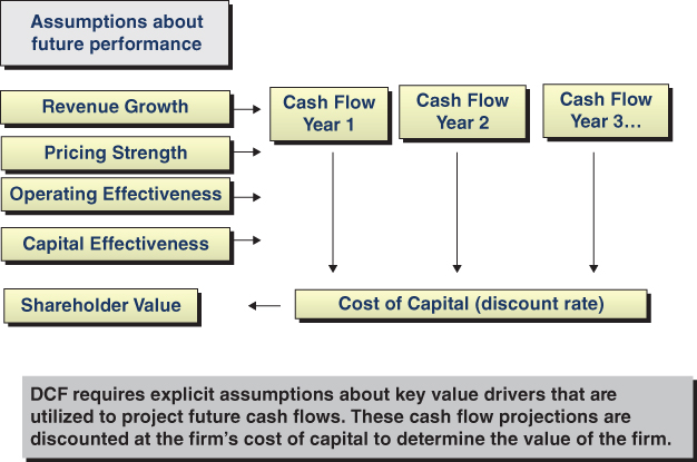
FIGURE 22.1 Discounted Cash Flow (DCF)
A sample worksheet for a DCF valuation is presented in Table 22.1. This example builds on the Roberts Manufacturing Company (RMC) example introduced in Chapter 2, utilizing the financial performance and other information presented in Table 2.5. This DCF valuation worksheet was developed for the primary purpose of understanding the overall dynamics of a firm's valuation, and may require modification to be used to as a valuation tool. For example, the model uses a single estimate of future sales growth and other key variables. Generally, a valuation would be based on estimates of key financial inputs for each period, supported by detailed projections and assumptions.
TABLE 22.1 DCF Valuation Model ![]()
 |
At first glance, the model presented in Table 22.1 can be overwhelming. We will review the model by breaking it into six key steps:
- Review and present the firm's financial history.
- Project future cash flows by estimating key elements of future operating performance.
- Estimate the terminal or postplanning horizon value.
- Discount the cash flows.
- Estimate the value of the firm.
- Explore the dynamics of the valuation.
Step 1: Include and Review the Firm's Financial History
While the DCF valuation will be based on expected future cash flows, it is essential to review and consider recent history and trends in developing the projected financial results. The DCF model should present three or four years of history alongside the projections. In addition to providing a base from which the preparer estimates future cash flows, it provides a basis for others to evaluate the future projections in the context of recent performance. For example, if sales have grown at 3% to 5% over the past several years, why are we projecting 8% growth over the next several years?
Step 2: Project Future Cash Flows by Estimating Key Elements of Future Operating Performance
After reviewing the historical performance and identifying the key drivers of current and future performance, the analyst or manager can project the expected future financial performance. It is deceptively easy to plug in estimated sales, margins, expenses, and so forth, to arrive at financial projections and estimated cash flows. However, significant analysis, understanding, and thought are required to project key variables such as revenue or gross margins. For example, to predict revenue for a firm, multiple factors must be considered, including:
- Economic factors (growth, recession, etc.)
- Market size and growth
- Competitive factors
- Unit volume
- Pricing trends
- Product mix
- Customer success
- New product introduction
- Product obsolescence
It is extremely important to document the critical assumptions about revenue and all other key elements of financial performance. These assumptions can then be evaluated, changed, monitored, and “flexed” to understand the significance of each in the estimated value of the firm. Since no one has a crystal ball, we know that actual results will vary from our projections. Much of the value in business planning results from the process of planning, as opposed to the plan or financial projection itself. Additional information on developing long‐term projections is contained in Chapter 14.
Another critical decision in DCF valuations is to determine the forecast horizon, the period for which we project future financial performance in detail. In theory, a company has an extended, if not infinite, life. However, it typically is not practical or necessary to attempt to forecast financial results for 20 or 30 years. The forecast horizon selected should vary according to the individual circumstances. Most discounted cash flow estimates for ongoing businesses will determine the value of the projected cash flows for the forecast horizon (5 to 10 years) and will then add to that an estimate of the value of the business at the end of that period, called the “terminal value” (TV) or “post‐horizon value.”
Two key factors should be considered in setting the forecast horizon. First, ensure that there is a balance between the value of the cash flows generated during the forecast horizon and the estimated terminal value. If substantially all of the estimated value is attributable to the terminal value, the forecast horizon should be extended. The second and related consideration is to extend the forecast horizon to a point where the financial performance reaches a sustainable or steady‐state basis. For example, if a firm is in a period of rapid growth, the cash flows at the end of the horizon will still reflect significant investments in expenses, working capital, and equipment. The forecast horizon should extend beyond this rapid growth phase to a point beyond where it reaches a long‐term sustainable growth rate. This will ensure that the key variables impacting cash flow reach a steady state, allowing this to be used as a base for estimating the terminal value.
Step 3: Estimate the Terminal or Post–Planning Horizon Value
The use of a terminal value or post‐horizon value is an effective practical alternative to very long forecast horizons, subject to proper application. First, the factors in setting the forecast horizon as just described must be utilized. Second, care must be exercised in selecting the multiple or valuation technique utilized in calculating the terminal value. The terminal value is usually estimated by using one of two methods:
The first method involves taking the base performance in the past year (or average of the past several years) and estimating the value of the firm by applying a multiple to earnings or sales – for example, taking the final estimated earnings in year 2025 of $18,324 and applying a multiple of 16× to arrive at an expected terminal value of $293,190. Multiples could be applied in this manner to EBIT, EBITDA, and sales, as well as cash flow.
In the second method, the economic value of cash flows is determined beyond the forecast horizon by assuming that the cash flows will continue to be generated at the level of the last projected year, forever. More common is to assume that the future cash flows will continue to grow from the last projected year at some level, say 3% to 5%, in perpetuity.
Assuming no future growth beyond 2025, the estimated value of annual cash flows of $13,526 continuing in perpetuity is:
For Roberts Manufacturing Company:

Assuming future growth after 2025 at g%:
For Roberts Manufacturing Company:

Since a case can be made supporting both methods, I recommend computing a range of estimated terminal values using both multiples and economic value. Understanding the underlying reasons for the different values is informative and should be explored. One of the estimates must ultimately be selected and used for the terminal value. Since the estimate of TV is usually significant to the overall valuation, a sensitivity analysis using multiple estimates of the terminal value should be created. This analysis should provide a more comprehensive understanding of the impact of key assumptions on the valuation of the company.
Common mistakes in estimating the terminal value include using inappropriate price‐earnings (P/E) multiples or unrealistic post‐horizon growth rates. The P/E multiple used in the TV estimate should be consistent with the performance estimated for the post‐horizon growth period. This may be significantly different from current P/E ratios reflecting current performance. Post‐horizon growth rates should be modest, since perpetuity means forever! Few companies achieve high levels of growth over extended periods, and many companies' growth rates slow to overall economic growth levels or even experience declines in sales over time.
Step 4: Discount the Cash Flows
Discounted cash flow (DCF) can be utilized to estimate the total value of the firm or the value of equity. Typically, we will estimate the total value of the firm by projecting total cash flows available to all investors, both equity and debt. We will then discount the cash flows at the weighted average cost of capital (WACC), which is an estimate of the returns expected by investors. Discount rates and the cost of capital are explored in greater detail in Chapter 19.
Step 5: Estimate the Value of the Firm and Equity
The resultant discounted cash flow is the total value of the firm, also referred to as the enterprise value (EV). To compute the value of equity, two adjustments must be considered. First, if the firm has a substantial cash reserve, this adjustment is added to the discounted value of projected cash flows. Second, in order to compute the value of equity, we deduct the value of the debt. The estimated value of an individual share can then be determined by dividing the market value of equity by the number of shares outstanding. Where there are significant stock options or other common stock derivatives outstanding, these should also be considered in the share count. In some cases, analysts may also make an adjustment to reflect the absence of ready liquidity for smaller privately owned enterprises.
Step 6: Explore the Dynamics of the Valuation
Arguably the most important part of valuing a business is to explore, evaluate, and communicate the dynamics of the valuation. This can be accomplished by performing sensitivity analysis, scenario analysis, and value decomposition using DCF. One of the criticisms of discounted cash flow analysis is that it requires assumptions about the future. In my view, this is a major strength of DCF analysis. We all recognize that it is not possible to predict the future, including specific projections of sales, costs, and numerous additional variables required for completing a thorough DCF analysis.
Sensitivity Analysis. By using sensitivity analysis, we can identify and quantify the sensitivity of shareholder value to key assumptions. The analysis allows us to identify the most critical factors impacting the value of a firm, such as revenue growth and profitability. Using the DCF worksheet, the analyst can change or flex key assumptions such as sales growth and profitability, and record the resultant value. The results can then be summarized as illustrated in Table 22.2.
TABLE 22.2 DCF Sensitivity Analysis ![]()
| DCF Value Sensitivity Analysis | ||||||
| Stock Price | ||||||
| Roberts Manufacturing Co. | Sales Growth Rate | |||||
| 4% | 6% | 8% | 10% | 12% | ||
| 20.0% | $12.11 | $13.49 | $15.04 | $16.80 | $18.77 | |
| 17.5% | 10.52 | 11.68 | 13.00 | 14.49 | 16.17 | |
| Operating Income % | 15.0% | 8.92 | 9.88 | 10.96 | 12.18 | 13.56 |
| 12.5% | 7.33 | 8.08 | 8.92 | 9.87 | 10.95 | |
| 10.0% | 5.74 | 6.27 | 6.88 | 7.57 | 8.34 | |
Scenario Analysis. While sensitivity analysis is simply a math exercise to determine the effect of changing specific assumptions, scenario analysis requires that a different “story” be told. The base or primary case undoubtedly contains critical assumptions about product introductions, competitor and customer actions and performance, the economy, and many others.
Under each scenario, multiple assumptions must be revisited. For example, a recession might affect sales volume and pricing, and may also reduce material and labor costs.
For Roberts Manufacturing Company, additional scenarios could be created. Each scenario would be supported by a financial projection that would be used to revalue the enterprise.
Value Decomposition. Using our DCF model, we can decompose or estimate the contribution to total value of any specific variable. For example, I find it useful to highlight the value of current performance for an enterprise versus the value associated with improvements to performance, including future growth and profitability improvements (see Figure 22.2). The value of current performance levels (i.e. assuming that the current cash flow remains constant in perpetuity) can be estimated using the formula for an annuity in perpetuity introduced in Chapter 19.


FIGURE 22.2 Value Decomposition 
This value compares to our DCF valuation of $188,408, indicating that a disproportionate amount of the valuation is associated with assumptions about improved performance in the projections. In the Roberts Manufacturing case, this improvement is due to the assumption of 8% growth per year (all other assumptions are held constant).
ESTIMATING THE VALUE OF FIRMS BY USING THE VALUATION OF SIMILAR FIRMS: MULTIPLES OF REVENUES, EARNINGS, AND RELATED MEASURES
The other commonly used valuation technique is based on using measures of revenues, earnings, or cash flow and capitalizing these amounts using a multiplier that is typical for similar companies. These methods are essentially shortcuts or rules of thumb based on economic theory. Users of these methods tend to establish ranges for certain industries. For example, retail companies may trade at a multiple of 0.5 to 1.0 times revenues, while technology companies may trade at 2 to 3 times revenues, or higher. The significant difference between the multiples for the two industries is explained by many factors that are independent of the current revenue level. For example, expected growth in revenues, profitability, risk, and capital requirements will have an impact on the revenue multiple. The use of multiples is common among operating executives and bankers as an easily understood basis for valuation. It also facilitates comparing relative valuations across companies.
In applying multiples, it is important to use consistent measures of income and valuation. Specifically, we must determine if we are attempting to estimate the value of the firm (enterprise value) or the value of the equity. To illustrate these techniques, we will use the information provided in Table 2.5 for Roberts Manufacturing Company.
Price‐to‐Sales Ratio
The price‐to‐sales ratio computes the value of the firm divided by the estimated or recent sales levels.
For example, Roberts Manufacturing Company has sales of $100 million and an estimated (enterprise) value of $190 million (debt of $10.0 million and equity of $180.0 million).

Other companies in this industry have price‐to‐sales ratios of 1.3 to 2.0. This would indicate a comparable valuation range of $130 million to $200 million for Roberts Manufacturing Company. The value‐to‐sales ratio for Roberts Manufacturing Company is within the range of similar or comparable companies, although at the high end of that range.
Advantages: The price‐to‐sales ratio is a simple, high‐level measure.
Disadvantages/Limitations: The measure requires many implicit assumptions about key elements of financial performance, including growth rates, margins, capital requirements, and capital structure.
Price‐Earnings (P/E) Ratio
The price‐earnings (P/E) ratio compares the price of the stock to the firm's earnings. Using per‐share information, the P/E ratio is calculated as follows:

For Roberts Manufacturing Company:

The valuations of companies comparable to Roberts Manufacturing Company indicate a P/E ratio range of 16 to 20 times earnings. Roberts Manufacturing Company's stock price of $10.59 is within the range indicated by the market research ($8.94 to $11.18) using the comparable P/E range.
This measure can also be computed at the firm level:

Advantages: This method is simple to employ and commonly used in practice.
Disadvantages and Limitations: Several problems exist with this technique. First, earnings are accounting measures and not directly related to economic performance or cash flows. This has become an increasing problem in recent years as accounting profit continues to diverge from the underlying economic performance. Second, this measure also requires many implicit assumptions about key elements of financial performance, including growth rates, capital requirements, and capital structure.
Enterprise Value/Earnings before Interest and Taxes (EBIT)
This method compares the total value of the firm to the earnings before interest and taxes. Recall that EBIT generally approximates operating income. Since it is a measure of income before deducting interest expense, it represents income available to all investors, both equity (shareholders) and debt (bondholders). Therefore, we will compare this measure to the total value of the firm (EV).

For Roberts Manufacturing Company:

Advantages: This method is also simple to use. It results in valuations based on earnings available to all investors.
Disadvantages and Limitations: This method does not directly take into account other key elements of performance, such as growth or capital requirements.
Enterprise Value/EBITDA
This measure is very close to EV/EBIT, but uses EBITDA as a better approximation of cash flow, since it adds back the noncash charges, including depreciation and amortization (D&A).
For Roberts Manufacturing Company:

Other similar companies are valued at 8 to 10 times EBITDA. Based on ratios for comparable companies, Roberts Manufacturing Company is valued just outside the high end of this range.
Advantages: This method is simple to apply and is based on an approximation of cash flow.
Disadvantages and Limitations: The primary limitation with this method is that it does not explicitly account for growth or future capital requirements.
Price‐Earnings Growth or “PEG” Ratio
The price‐earnings growth (PEG) ratio is a derivative of the price‐earnings ratio that attempts to factor in the impact of growth in price‐earnings multiples. The logic here is that there is a strong correlation between growth rates and P/E multiples. Companies with higher projected growth rates of earnings, for example technology companies, should have higher P/E ratios than firms with lower expected growth rates.
The PEG ratio is computed as follows:

For Roberts Manufacturing Company:

Roberts Manufacturing Company has a very high PEG ratio relative to the peer group. This may reflect a number of factors: perhaps strong cash flows, or consistent operating performance relative to the benchmark group.
Advantages: This method reflects a key driver of valuation: expected growth.
Disadvantages and Limitations: Again, this measure does not directly reflect other key elements of financial performance.
BUILDING SHAREHOLDER VALUE IN A MULTIPLES FRAMEWORK
Many investors, analysts, and managers use multiples of earnings in investment and valuation decisions. Using multiples, there are two ways to build value. First, the firm can improve the base performance measure, for example earnings. The second way is to command a higher multiple. For illustration, let's assume that Roberts Manufacturing Company's valuation is being driven by capitalizing earnings (P/E ratio). The stock is valued at $10.59 because the firm earned $0.56 per share in earnings and the market has capitalized those earnings at approximately 19 times. The price of Roberts Manufacturing Company stock will rise when the earnings increase and/or if the market applies a higher multiple, for example increasing to 22 times earnings. In the latter case, the stock would trade at $12.32 (22 × $0.56).
Factors That Affect Multiples
What factors would cause the multiples to expand or contract? A variety of factors can contribute, including some specific to the firm and others that relate to the industry or even the general economy. Examples include expected growth rates, the quality of earnings, cash generation, perceived risk, and interest rates. A firm's P/E multiple should expand if it demonstrates a higher expected growth rate, improved working capital management, and/or more consistent operating performance. It will likely contract if it consistently misses financial targets, utilizes capital less effectively, or increases the perceived risk by entering a new market. In addition, economic factors such as changes in interest rates or expected economic conditions will cause multiples to expand or contract.
Use of Multiples in Setting Acquisition Values
Most of the multiples used in the previous discussion are typically derived from the valuation of other similar companies, industry averages, or broad market indexes. This is commonly referred to as the “trading multiple” – that is, the value set by trades in the equity markets. If a company is being considered as a potential acquisition target, the multiples will typically be adjusted to reflect a likely control or acquisition premium. These acquisition values are referred to as transaction values versus trading values, and the multiples would be derived by looking at transactions involving similar companies. Control premiums are typical for two reasons. First, boards and management teams are unlikely to surrender control of a company unless there is an immediate reward to the selling shareholders. In addition, the acquirer should be able to pay more than a passive investor, since it will be able to control the company and should be able to realize a higher growth in earnings and cash flow due to synergies with the acquiring company. Valuation for acquisition purposes is covered in Chapter 23, Analysis of Mergers and Acquisitions.
Trailing and Forward Multiples
When applying multiples of earnings, sales, and other measures, the analyst must select a base period. The value of the multiple will vary depending on whether the multiple is applied to actual past results (e.g. “trailing 12 months earnings”) or a future period's estimated performance (e.g. “forward 12 months earnings”). The multiple applied to trailing earnings will be higher than the multiple applied to future earnings for two reasons: risk and the time value of money. There is risk associated with future earnings projections; they may not be achieved. The time value of money suggests that a dollar to be received next year is not worth a dollar today. These two factors result in a discount of the multiples used for future periods.
Adjusting or Normalizing the Base
Using multiples requires us to use a measure for a single period, typically a year. Many of the measures, such as sales or earnings, for the selected period may have been or are anticipated to be significantly impacted by a number of anomalous, or one‐time, factors. For example, the current year earnings may include income that is not expected to continue into the future. Or perhaps the income includes a so‐called nonrecurring adjustment to record a legal settlement or the closing of a plant. In these situations, companies and analysts may adjust the base to normalize the earnings, often referred to as pro forma or non‐GAAP earnings.
This practice became very prevalent in the 1990s and led to a number of abuses. Certain companies were accused of being selective in choosing items to exclude, leading to a perceived overstatement of the earnings on a pro forma basis. The Securities and Exchange Commission subsequently placed significant constraints on reporting adjusted earnings. Several reasons gave rise to the use of pro forma measures:
- Deficiencies in Generally Accepted Accounting Principles (GAAP). There has been a continuing divergence between GAAP accounting measures and economic results. Specific issues relate to accounting for acquisitions, income taxes, stock options, and pension plans.
- Significant Restructuring, Divestitures, and Acquisitions. One‐time or nonrecurring charges are reflected in earnings in a specific period based on very precise rules established by the accounting rule makers. However, a significant restructuring may be viewed as an investment for economic and valuation purposes. Acquisitions and divestitures may result in a disconnect between historical performance trends and future projections.
Some advocate using other measures, such as cash flow or economic profit, which adjust the accounting earnings to a measure with greater relevance in evaluating the economic value and performance of the firm.
Problems with Using Multiples
The use of multiples has several inherent limitations, especially for our purposes in linking shareholder value to operating performance.
- Circular reference. The basic logic with multiples is that one company's value is determined by looking at the valuation of other companies. This is very useful in comparing relative valuations and in testing the fairness of a company's valuation. Management teams and boards rely heavily on the use of multiples to review the fairness of acquisition prices. However, if the industry or peer group is overvalued, then this method will result in overvaluing the subject enterprise. This was a contributing factor to the technology/Internet (and other) market bubbles. The logic was that since dot.com1 was valued at 50 times sales, so should dot.com2, notwithstanding the fact that neither valuation was supported by basic economic fundamentals.
- Implicit performance assumptions. Another problem with this methodology is that it is not directly related to key value drivers or elements of financial performance. It is very difficult to understand the assumptions underlying values computed using multiples. If a firm is valued at 18 times earnings, what are the underlying assumptions for revenue growth, working capital requirements, and other similar factors? The market often attempts to cope with this limitation by increasing or decreasing the multiple over benchmarks to reflect factors such as consistency of performance, quality of earnings, lower or higher risk, and so forth. Such stocks would be described as “trading at a premium to the market based on” certain identified factors.
- Selecting appropriate comparables. Using multiples requires the analyst to select a set of comparable companies or a peer group. This can be a significant challenge. Few companies are so‐called pure plays that are serving a single industry or match up closely with other companies. Further, choosing an appropriate benchmark or peer group can lead to great debates, since the process is both subjective and often emotionally charged.
INTEGRATED VALUATION SUMMARY FOR ROBERTS MANUFACTURING COMPANY
The individual valuation techniques described in this chapter should be combined to form a summary analysis of estimated valuation for Roberts Manufacturing Company. Each measure contributed a view of valuation that contributes to an overall picture. The numerical summary shown in Table 22.3 can be converted into a more user‐friendly visual summary in Figure 22.3.
TABLE 22.3 Roberts Manufacturing Company Valuation Summary Table ![]()
| Valuation Analysis: Multiples | |||||
| Benchmark Range | |||||
| Value Basis | Roberts | Low | High | ||
| Sales | 2018 Result | $100,000 | |||
| Multiple | 1.9 | 1.3 | 2.0 | ||
| Enterprise | Value/Indicated Range | $190,030 | $130,000 | $200,000 | |
| Equity | Value/Indicated Range | $180,030 | $120,000 | $190,000 | |
| Earnings | 2018 Result | $9,501 | |||
| Multiple | 18.95 | 16 | 20 | ||
| Equity | Value/Indicated Range | $180,030 | $152,011 | $190,014 | |
| Per Share | 10.59 | 8.94 | 11.18 | ||
| EBITDA | 2018 Result | $18,750 | |||
| Multiple | 10.13 | 8.00 | 10.00 | ||
| Enterprise | Value/Indicated Range | $190,030 | $150,000 | $187,500 | |
| Equity | Value/Indicated Range | $180,030 | $140,000 | $177,500 | |
| Price‐Earnings | P/E | 18.95 | |||
| Growth | Estimated Growth (%) | 8 | |||
| PEG | 2.37 | 1.3 | 2.0 | ||
| DCF | Equity | Value | $186,352 | NA | NA |

FIGURE 22.3 Roberts Manufacturing Company Valuation Summary Graph
Roberts Manufacturing Company's current value is at the high end of the 12‐month trading range and near or exceeding the top of the range for comparable companies. In this case, it would be important to understand the underlying performance characteristics of the benchmark group compared to Roberts Manufacturing Company. Is Roberts Manufacturing Company's valuation supported by better performance or higher future expectations of growth? The current market value approximates our estimate of the DCF value. This indicates that the market is probably expecting future performance in line with our projections used in the DCF.
Comprehensive Valuation Summary
For fans of dashboards or one‐page recaps, the comprehensive valuation summary (Figure 22.4) may be of interest. It combines a number of the tools we have reviewed in the chapter to present a very comprehensive view into the dynamics of the valuation of this company.

FIGURE 22.4 Valuation Summary
VALUE DRIVERS
The fundamental objective for most companies is to create value for shareholders. For these enterprises, we have successfully utilized a framework that links value creation and value drivers to key business processes and activities.
In Chapter 7, we introduced the value performance framework (VPF) (Figure 22.5) as one of several options to establish an overall framework for performance management. The VPF identifies six drivers of shareholder value:

FIGURE 22.5 The Value Performance Framework
- Sales growth
- Relative pricing strength
- Operating effectiveness
- Capital effectiveness
- Cost of capital
- The intangibles
Factors such as interest rates, market conditions, and irrational investor behavior will, of course, affect the price of a company's stock. However, the six value drivers identified are those that management teams and directors can drive to build long‐term sustainable shareholder value.
It is important to recognize that the significance of each driver will vary from firm to firm and will also vary over time for a particular firm. For example, a firm with increased competition in a low‐growth market will likely place significant emphasis on operating and capital effectiveness. In contrast, a firm with a significant opportunity for sales growth is likely to focus on that driver and place less emphasis on capital management or operating effectiveness. At some time in the future, however, this high‐growth firm may have to deal with a slower growth rate and may have to shift emphasis to other drivers, such as operating efficiency and capital management.
In order to attain its full potential value, a firm must understand the potential contribution of each driver to shareholder value. It starts with the six value drivers that ultimately determine shareholder value. Underneath these value drivers are some of the key activities and processes that determine the level of performance in each value driver. In addition, the framework identifies some of the key performance indicators that can be used to measure the effectiveness of these activities and processes. For example, sales growth is a key driver of shareholder value. A subset of sales growth is the level of organic growth, excluding the impact on sales growth of any acquisitions. Organic sales growth will be driven by a number of factors, including customer satisfaction, which can be tracked by key metrics such as on‐time deliveries (OTDs) and the level of past‐due orders.
In order to create a linkage between the day‐to‐day activities of the employees and the company's share value, we must first create a discounted cash flow (DCF) model for the company. We can start with the model introduced in this chapter. We first input several years of historical performance as a baseline, and then project key elements of the expected future performance. The projections should be based on our best estimate of future performance. The projections should be realistic and should be reviewed against the recent historical performance trends experienced by the firm. This scenario, using our projections for the future performance, can be described as the “base forecast.”
If the firm is publicly traded, the preliminary valuation can be tested against the current stock price. If the value indicated by the DCF model is significantly different from the recent trading range of the stock, one or more of your assumptions is likely to be inconsistent with the assumptions held by investors and potential investors. Identifying and testing the critical assumptions that investors are making in valuing the firm's stock can be very enlightening. The DCF model will allow you to easily change key assumptions and observe the potential impact on the value of the stock. It is very informative to iterate key assumptions until you can achieve a valuation consistent with recent market values for your company. For firms that are not publicly traded, this process can be performed for a comparable firm or firms that are in the same industry. Growth rates, other key drivers, and valuation metrics can then be transferred to the private firm to understand value drivers and expectations for the industry.
After developing a perspective on valuation and value drivers, the second step is to identify the critical activities and processes that impact each value driver. While many of these critical processes and activities are common from business to business, their relative importance will vary significantly among companies. Further, every industry and firm has certain unique characteristics that must be identified and reflected in the framework. In Chapters 15 through 19, we examined each of the value drivers and linked those drivers to critical processes and activities.
This framework allows managers to evaluate potential improvement projects and identify high‐leverage opportunities in the context of value creation. Too often, companies or functional managers embark on initiatives to improve certain aspects of the business without fully considering the impact on value creation. Will the initiatives be worth the investment of time and valuable resources? The VPF allows managers to rank various programs and address the following questions:
- How much value will be created if we accelerate sales growth from 5% to 10%?
- How much value will be created if we reduce manufacturing defects by 20%?
- How much value will be created if we reduce accounts receivable days sales outstanding (DSO) from 65 to 50 days? If we improve inventory turns from 4 to 6?
- Which of these programs will have the greatest impact on value?
Identifying High‐Leverage Improvement Opportunities and Estimating Full Potential Value
Utilizing the tools of business process assessment, benchmarking, and discounted cash flow analysis, managers can estimate the potential improvements in the value drivers and quantify the effect on the value of the firm if the targeted performance is achieved. We start with the benchmarking summary developed in Chapter 11 (see Table 22.4).
TABLE 22.4 Benchmarking Summary ![]()
| Benchmarking Summary and Target Worksheet | ||||||
| Best in | Best | Performance | ||||
| Roberts Co. | Median | Top Quartile | Class | Practice | Target | |
| Revenue Growth | 8.0% | 8.0% | 12.0% | 15.0% | 25.0% | 12.0% |
| Gross Margin % | 55.0% | 52.0% | 56.0% | 60.0% | 56.0% | |
| Operating Expenses | 40.0% | 40.0% | 38.0% | 35.0% | 38.0% | |
| Operating Margins | 15.0% | 12.0% | 18.0% | 20.0% | 25.0% | 18.0% |
| Tax rate | 34.0% | 30.0% | 25.0% | 15.0% | 10.0% | 25.0% |
| Operating Capital % Sales | 30.0% | 25.0% | 15.0% | 10.0% | 15.0% | 15.0% |
| WACC | 11.99% | 10.59% | 10.13% | 9.77% | 9.07% | 10% |
| Cost of Equity | 12.4% | 11.3% | 11.0% | 10.7% | 9.8% | |
| Beta | 1.24 | 1.05 | 1.00 | 0.95 | 0.80 | |
| Debt to Total Capital | ||||||
| Book | 15.3% | 30.0% | 40.0% | 50.0% | 50.0% | |
| Market | 5.3% | 10.0% | 13.3% | 16.7% | 16.7% | |
In this case, Roberts Manufacturing Company has set preliminary performance targets to achieve top‐quartile performance in each key measure in Table 22.4. Using the DCF model, the value created by each change can be estimated. The value of the firm could be increased from $196.4 million to $389 million if each of the performance improvements is realized. (See Table 22.5.) This may be a good place to start, but requires additional vetting. The targets should be refined by evaluating processes and operating effectiveness and testing the relative impact on value creation to develop a target business model. This exercise is not meaningful unless the team has a plan for how these improvements will be achieved.
TABLE 22.5 Summary of Full Potential Value ![]()
| Enterprise | |||||
| From | To | Value | Increment | How? | |
| Current Value | 196.4 | Current Performance Expectations | |||
| Increase Sales Growth Rate | 8% | 12% | 241 | 44.6 | Improve Quality and On‐Time Delivery |
| Improve Gross Margin % | 55% | 56% | 259 | 18 | Reduce Material Costs |
| Reduce Operating Expenses | 40% | 38% | 294 | 53 | Process Initiatives |
| Reduce Tax Rate | 34% | 25% | 338 | 97 | Tax Benefits from New Manufacturing Facility |
| Reduce Operating Capital % | 30% | 15% | 352 | 111 | Improve Supply Chain and Revenue Process |
| Reduce WACC | 12% | 10% | 389 | 148 | Improve Forecasting and Change Capital Structure |
A graphic presentation of this analysis is shown in Figure 22.6.
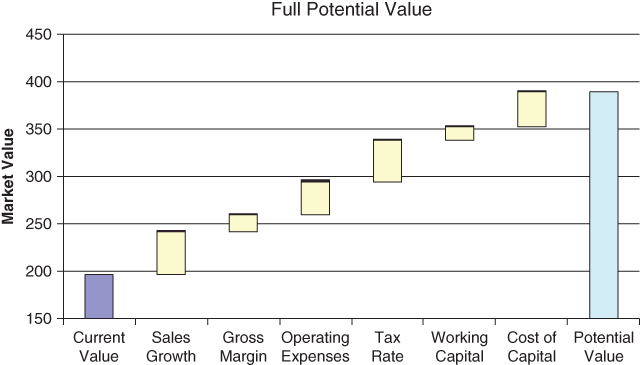
FIGURE 22.6 Estimating Full Potential Valuation
Projecting improved performance on spreadsheets is very easy. Achieving these improvements in actual results requires substantial planning, effort, and follow‐through. Central to achieving these performance goals is the selection and development of effective performance measures.
SUMMARY
While each of the valuation techniques has limitations, they do provide insight from a variety of perspectives. It is best to use a combination of measures and techniques in reviewing the valuation of a firm. When an analyst summarizes these measures for a firm and compares them to key benchmarks, significant insights can be gained. Conversely, inconsistencies across the valuation measures for a company are worth exploring and can usually be explained by identifying a specific element of financial performance that the measure doesn't reflect. For example, a company that consistently meets or exceeds operating plans and market expectations will typically be afforded a higher P/E multiple than its peers, and the company will trade at a premium to the industry norms.
Managers can use the DCF valuation model to estimate potential growth in value resulting from improving performance across key value drivers.
Given this foundation in valuation, we will turn our attention to unique issues in analyzing and valuing mergers and acquisitions in Chapter 23.