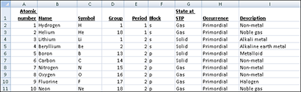
Figure 12-1: A spreadsheet with elements of the periodic table serves as our example throughout this chapter.
Chapter 12
Getting Data into and out of R
In This Chapter
![]() Exploring the various ways of getting data into R
Exploring the various ways of getting data into R
![]() Looking at how to save your results
Looking at how to save your results
![]() Understanding how files are organized in R
Understanding how files are organized in R
Every data-processing or analysis problem involves at least three broad steps: input, process, and output. In this chapter, we cover the input and output steps.
In this chapter, we look at some of the options you have for importing your data into R, including using the Clipboard, reading data from comma-separated value (CSV) files, and interfacing with spreadsheets like Excel. We also give you some pointers on importing data from commercial software such as SPSS. Next, we give you some options for exporting your data from R. Finally, you get to manipulate files and folders on your computer.
Getting Data into R
You have several options for importing your data into R, and we cover those options in this section.
Because spreadsheets are so widely used, the bulk of this chapter looks at the different options for importing data originating in spreadsheets. To illustrate the techniques in this chapter, we use a small spreadsheet table with information about the first ten elements of the periodic table, as shown in Figure 12-1.
Entering data in the R text editor
Although R is primarily a programming language, R has a very basic data editor that allows you to enter data directly using the edit() function.
 The
The edit() function is only available in some R code editors, so depending on which software you’re using to edit your R code, this approach may not work. As of this writing, this option is not yet supported by RStudio.
To use the R text editor, first you need to initiate a variable. For example, to create a data frame and manually enter some of the periodic table data, enter the following:
elements <- data.frame()
elements <- edit(elements)
This displays an interactive editor where you can enter data, as shown in Figure 12-2. Notice that because the data frame is empty, you can scroll left and right, or up and down, to extend the editing range. Notice also that the editor doesn’t allow you to modify column or row names.
Figure 12-2: Editing data in the R interactive text editor.

Enter some data. Then to save your work, click the X in the top-right corner.
To view the details that you’ve just entered, use the print() function:
> print(elements)
var1 var2 var3
1 1 Hydrogen H
2 2 Helium He
3 3 Lithium Li
Using the Clipboard to copy and paste
Another way of importing data interactively into R is to use the Clipboard to copy and paste data.
 If you’re used to working in spreadsheets and other interactive applications, copying and pasting probably feels natural. If you’re a programmer or data analyst, it’s much less intuitive. Why? Because data analysts and programmers strive to make their results reproducible. A copy-and-paste action can’t be reproduced easily unless you manually repeat the same action. Still, sometimes copying and pasting is useful, so we cover it in this section.
To import data from the Clipboard, use the readClipboard() function. For example, select cells B2:B4 in the periodic table spreadsheet, press Ctrl+C to copy those cells to the Clipboard, and then use the following R code:
> x <- readClipboard()
> x
[1] “Hydrogen” “Helium” “Lithium”
As you can see, this approach works very well for vector data (in other words, a single column or row of data). But things get just a little bit more complicated when you want to import tabular data to R.
To copy and paste tabular data from a spreadsheet, first select a range in your sheets (for example, cells B1:D5). Then use the readClipboard() function and see what happens:
> x <- readClipboard()
> x
[1] “Name Symbol Group” “Hydrogen H 1” “Helium He 1”
[4] “Lithium Li 1” “Beryllium Be 2”
This rather unintelligible result looks like complete gibberish. If you look a little bit closer, though, you’ll notice that R has inserted lots of “ ” elements into the results. The “ ” is the R way of indicating a tab character — in other words, a tab separator between elements of data. Clearly, we need to do a bit more processing on this to get it to work.
The backslash in “ ” is called an escape sequence. See the sidebar “Using special characters in escape sequences,” later in this chapter, for other examples of frequently used escape sequences in R.
The very powerful read.table() function (which you get to explore in more detail later in this chapter) imports tabular data into R. You can customize the behavior of read.table() by changing its many arguments. Pay special attention to the following arguments:
![]()
file: The name of the file to import. To use the Clipboard, specify file = “clipboard”.
![]()
sep: The separator between data elements. In the case of Microsoft Excel spreadsheet data copied from the Clipboard, the separator is a tab, indicated by “ ”.
![]()
header: This argument indicates whether the Clipboard data includes a header in the first row (that is, column names). Whether you specify TRUE or FALSE depends on the range of data that you copied.
![]()
stringsAsFactors: If TRUE, this argument converts strings to factors. It’s FALSE by default.
> x <- read.table(file = “clipboard”, sep = “ ”, header=TRUE)
> x
Name Symbol Group
1 Hydrogen H 1
2 Helium He 1
3 Lithium Li 1
4 Beryllium Be 2
 Although R offers some interactive facilities to work with data and the Clipboard, it’s almost certainly less than ideal for large amounts of data. If you want to import large data files from spreadsheets, you’ll be better off using CSV files (described later in this chapter).
Note: Unfortunately, readClipboard() is available only on Windows.
Using special characters in escape sequences
Certain keys on your keyboard, such as the Enter and Tab keys, produce behavior without leaving a mark in the document. To use these keys in R, you need to use an escape sequence (a special character preceded by a backslash).
Here are some escape sequences you may encounter or want to use:
![]() New line:
New line:
![]() Tab stop:
Tab stop:
![]() Backslash:
Backslash: \
![]() Hexadecimal code:
Hexadecimal code: xnn
The new line (
) character comes in handy when you create reports or print messages from your code, while the tab stop ( ) is important when you try to read some types of delimited text file.
For more information, refer to the section of the R online manual that describes literal constants: http://cran.r-project.org/doc/manuals/R-lang.html#Literal- constants.
Reading data in CSV files
One of the easiest and most reliable ways of getting data into R is to use text files, in particular CSV files. The CSV file format uses commas to separate the different elements in a line, and each line of data is in its own line in the text file, which makes CSV files ideal for representing tabular data. The additional benefit of CSV files is that almost any data application supports export of data to the CSV format. This is certainly the case for most spreadsheet applications, including Microsoft Excel and OpenOffice Calc.
Some EU countries use an alternative standard where a comma is the decimal separator and a semicolon is the field separator.
In the following examples, we assume that you have a CSV file stored in a convenient folder in your file system. If you want to reproduce the exact examples, create a small spreadsheet that looks like the example sheet in Figure 12-1. To convert an Excel spreadsheet to CSV format, you need to choose File⇒Save As, which gives you the option to save your file in a variety of formats. Keep in mind that a CSV file can represent only a single worksheet of a spreadsheet. Finally, be sure to use the topmost row of your worksheet (row 1) for the column headings.
Using read.csv() to import data
In R, you use the read.csv() function to import data in CSV format. This function has a number of arguments, but the only essential argument is file, which specifies the location and filename. To read a file called elements.csv located at f: use read.csv() with file.path:
> elements <- read.csv(file.path(“f:”, “elements.csv”))
> str(elements)
‘data.frame’: 10 obs. of 9 variables:
$ Atomic.number: int 1 2 3 4 5 6 7 8 9 10
$ Name : Factor w/ 10 levels “Beryllium”,”Boron”,..: 6 5 7 1 2 3 9 10 4 8
$ Symbol : Factor w/ 10 levels “B”,”Be”,”C”,”F”,..: 5 6 7 2 1 3 8 10 4 9
$ Group : int 1 18 1 2 13 14 15 16 17 18
$ Period : int 1 1 2 2 2 2 2 2 2 2
$ Block : Factor w/ 2 levels “p”,”s”: 2 2 2 2 1 1 1 1 1 1
$ State.at.STP : Factor w/ 2 levels “Gas”,”Solid”: 1 1 2 2 2 2 1 1 1 1
$ Occurrence : Factor w/ 1 level “Primordial”: 1 1 1 1 1 1 1 1 1 1
$ Description : Factor w/ 6 levels “Alkali metal”,..: 6 5 1 2 4 6 6 6 3 5
R imports the data into a data frame. As you can see, this example has ten observations of nine variables.
 Notice that the default option is to convert character strings into factors. Thus, the columns
 Name, Block, State.At.STP, Occurrence, and Description all have been converted to factors. Also, notice that R converts spaces in the column names to periods (for example, in the column State.At.STP).
This default option of converting strings to factors when you use read.table() can be a source of great confusion. You’re often better off importing data that contains strings in such a way that the strings aren’t converted factors, but remain character vectors. To import data that contains strings, use the argument stringsAsFactors=FALSE to read.csv() or read.table():
> elements <- read.csv(file.path(“f:”, “elements.csv”), stringsAsFactors=FALSE)
> str(elements)
‘data.frame’: 10 obs. of 9 variables:
$ Atomic.number: int 1 2 3 4 5 6 7 8 9 10
$ Name : chr “Hydrogen” “Helium” “Lithium” “Beryllium” ...
$ Symbol : chr “H” “He” “Li” “Be” ...
$ Group : int 1 18 1 2 13 14 15 16 17 18
$ Period : int 1 1 2 2 2 2 2 2 2 2
$ Block : chr “s” “s” “s” “s” ...
$ State.at.STP : chr “Gas” “Gas” “Solid” “Solid” ...
$ Occurrence : chr “Primordial” “Primordial” “Primordial” “Primordial” ...
$ Description : chr “Non-metal” “Noble gas” “Alkali metal” “Alkaline earth metal” ...
If you have a file in the EU format mentioned earlier (where commas are used as decimal separators and semicolons are used as field separators), you need to import it to R using the read.csv2() function.
Using read.table() to import tabular data in text files
The CSV format, described in the previous section, is a special case of tabular data in text files. In general, text files can use a multitude of options to distinguish between data elements. For example, instead of using commas, another format is to use tab characters as the separator between columns of data. If you have a tab-delimited file, you can use read.delim() to read your data.
The functions read.csv(), read.csv2(), and read.delim() are special cases of the multipurpose read.table() function that can deal with a wide variety of data file formats. The read.table() function has a number of arguments that give you fine control over the specification of the text file you want to import. Here are some of these arguments:
![]()
header: If the file contains column names in the first row, specify TRUE.
![]()
sep: The data separator (for example, sep=”,” for CSV files or sep=” ” for tab-separated files).
![]()
quote: By default, strings are enclosed in double quotation marks (“). If the text file uses single quotation marks, you can specify this as the argument to quote (for example, quote=”’”, a single quote embedded between double quotes).
![]()
nrows: If you want to read only a certain number of rows of a file, you can specify this by providing an integer number.
![]()
skip: Allows you to ignore a certain number of lines before starting to read the rest of the file.
![]()
stringsAsFactors: If TRUE, it converts strings to factors. It’s FALSE by default.
You can access the built-in help by typing ?read.table into your console.
Reading data from Excel
If you ask users of R what the best way is to import data directly from Microsoft Excel, most of them will probably answer that your best option is to first export from Excel to a CSV file and then use read.csv() to import your data to R.
In fact, this is still the advice in Chapter 8 of the R import and export manual, which says, “The first piece of advice is to avoid doing so if possible!” See for yourself at http://cran.r-project.org/doc/manuals/R-data.html#Reading-Excel-spreadsheets. The reason is that many of the existing methods for importing data from Excel depend on third-party software or libraries that may be difficult to configure, not available on all operating systems, or perhaps have restrictive licensing terms.
However, since February 2011 there exists a new alternative: using the package XLConnect, available from CRAN at http://cran.r-project.org/web/packages/XLConnect/index.html. What makes XLConnect different is that it uses a Java library to read and write Excel files. This has two advantages:
![]() It runs on all operating systems that support Java.
It runs on all operating systems that support Java. XLConnect is written in Java and runs on Window, Linux, and Mac OS.
![]() There’s nothing else to load.
There’s nothing else to load. XLConnect doesn’t require any other libraries or software. If you have Java installed, it should work.
XLConnect also can write Excel files, including changing cell formatting, in both Excel 97–2003 and Excel 2007/10 formats.
To find out more about XLConnect, you can read the excellent package vignette at http://cran.r-project.org/web/packages/XLConnect/vignettes/XLConnect.pdf.
By now you’re probably itching to get started with an example. Let’s assume you want to read an Excel spreadsheet in your user directory called Elements.xlsx. First, install and load the package; then create an object with the filename:
> install.packages(“XLConnect”)
> library(“XLConnect”)
> excel.file <- file.path(“~/Elements.xlsx”)
Now you’re ready to read a sheet of this workbook with the readWorksheetFromFile() function. You need to pass it at least two arguments:
![]() file: A character string with a path to a valid
file: A character string with a path to a valid .xls or .xlsx file
![]() sheet: Either an integer indicating the position of the worksheet (for example,
sheet: Either an integer indicating the position of the worksheet (for example, sheet=1) or the name of the worksheet (for example, sheet=”Sheet2”)
The following two lines do exactly the same thing — they both import the data in the first worksheet (called Sheet1):
> elements <- readWorksheetFromFile(excel.file, sheet=1)
> elements <- readWorksheetFromFile(excel.file, sheet=”Sheet1”)
Working with other data types
Despite the fact that CSV files are very widely used to import and export data, they aren’t always the most appropriate format. Some data formats allow the specification of data that isn’t tabular in nature. Other data formats allow the description of the data using metadata (data that describes data).
The base distribution of R includes a package called foreign that contains functions to import data files from a number of commercial statistical packages, including SPSS, Stata, SAS, Octave, and Minitab. Table 12-1 lists some of the functions in the foreign package.
To use these functions, you first have to load the foreign package:
> library(foreign)
> read.spss(file=”location/of/myfile”)
Table 12-1 Functions to Import from Commercial Statistical Software Available in the foreign Package
|
System |
Function to Import to R |
|
SPSS |
|
|
SAS |
|
|
Stata |
|
|
Minitab |
|
Read the Help documentation on these functions carefully. Because data frames in R may have a quite different structure than datasets in the statistical packages, you have to pay special attention to how value and variable labels are treated by the functions mentioned in Table 12-1. Check also the treatment of special missing values.
These functions need a specific file format. The function read.xport() only works with the XPORT format of SAS. For read.mtp(), the file must be in the Minitab portable worksheet (.mtp) format.
Note that some of these functions are rather old. The newest versions of the statistical packages mentioned here may have different specifications for the format, so the functions aren’t always guaranteed to work.
Finally, note that some of these functions require the statistical package itself to be installed on your computer. The read.ssd() function, for example, can work only if you have SAS installed.
The bottom line: If you can transfer data using CSV files, you’ll save yourself a lot of trouble.
Finally, if you have a need to connect R to a database, then the odds are that a package exists that can connect to your database of choice. See the nearby sidebar, “Working with databases in R,” for some pointers.
Working with databases in R
Data analysts increasingly make use of databases to store large quantities of data or to share data with other people. R has good support to work with a variety of databases, but the exact details of how you do that will vary from system to system.
If you need to connect R to your database, a really good place to start looking for information is the Chapter 4 of the R manual “R data import/export.” You can read this chapter at http://cran.r-project.org/doc/manuals/R-data.html#Relational-databases.
The package RODBC allows you to connect to Open Database Connectivity (ODBC) data sources. You can find this package on CRAN at http://cran.r-project.org/web/packages/RODBC/index.html.
In addition, you can download and install packages to connect R to many database systems, including the following
![]() MySQL: The
MySQL: The RMySql package, available at http://cran.r-project.org/package=RMySQL
![]() Oracle: The
Oracle: The ROracle package, available at http://cran.r-project.org/package=ROracle
![]() PostgreSQL: The
PostgreSQL: The PostgreSQL package, available at http://cran.r-project.org/package=RPostgreSQL
![]() SQLite: The
SQLite: The RSQLite package, available at http://cran.r-project.org/package=RSQLite
Getting Your Data out of R
For the same reason that it’s convenient to import data into R using CSV files, it’s also convenient to export results from R to other applications in CSV format. To create a CSV file, use the write.csv() function. In the same way that read.csv() is a special case of read.table(), write.csv() is a special case of write.table().
To interactively export data from R for pasting into other applications, you can use writeClipboard() or write.table(). The writeClipboard() function is useful for exporting vector data. For example, to export the names of the built-in dataset iris, try the following:
> writeClipboard(names(iris))
This function doesn’t produce any output to the R console, but you can now paste the vector into any application. For example, if you paste this into Excel, you’ll have a column of five entries that contains the names of the iris data, as shown in Figure 12-3.
Figure 12-3: A spreadsheet after first using writeClipboard() and then pasting.

To write tabular data to the Clipboard, you need to use write.table() with the arguments file=”clipboard”, sep=” ”, and row.names=FALSE:
> write.table(head(iris), file=”clipboard”, sep=” ”, row.names=FALSE)
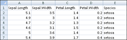
Again, this doesn’t produce output to the R console, but you can paste the data into a spreadsheet. The results look like Figure 12-4.
Figure 12-4: The first six lines of iris after pasting into a spreadsheet.
Working with Files and Folders
You know how to import your data into R and export your data from R. Now all you need is an idea of where the files are stored with R and how to manipulate those files.
Understanding the working directory
Every R session has a default location on your operating system’s file structure called the working directory.
You need to keep track and deliberately set your working directory in each R session. If you read or write files to disk, this takes place in the working directory. If you don’t set the working directory to your desired location, you could easily write files to an undesirable file location.
The getwd() function tells you what the current working directory is:
> getwd()
[1] “F:/git”
To change the working directory, use the setwd() function. Be sure to enter the working directory as a character string (enclose it in quotes).
This example shows how to change your working directory to a folder called F:/git/roxygen2:
> setwd(“F:/git/roxygen2”)
> getwd()
[1] “F:/git/roxygen2”
Notice that the separator between folders is forward slash (/), as it is on Linux and Mac systems. If you use the Windows operating system, the forward slash will look odd, because you’re familiar with the backslash () of Windows folders. When working in Windows, you need to either use the forward slash or escape your backslashes using a double backslash (\). Compare the following code:
> setwd(“F:\git\stringr”)
> getwd()
[1] “F:/git/stringr”
R will always print the results using /, but you’re free to use either / or \ as you please.
To avoid having to deal with escaping backslashes in file paths, you can use the file.path() function to construct file paths that are correct, independent of the operating system you work on. This function is a little bit similar to paste in the sense that it will append character strings, except that the separator is always correct, regardless of the settings in your operating system:
> file.path(“f:”, “git”, “surveyor”)
[1] “f:/git/surveyor”
It’s often convenient to use file.path() in setting the working directory. This allows you specify a cascade of drive letters and folder names, and file.path() then assembles these into a proper file path, with the correct separator character:
> setwd(file.path(“F:”, “git”, “roxygen2”))
> getwd()
[1] “F:/git/roxygen2”
You also can use file.path() to specify file paths that include the filename at the end. Simply add the filename to the path argument. For example, here’s the file path to the README.md file in the roxygen2 package installed in a local folder:
> file.path(“F:”, “git”, “roxygen2”, “roxygen2”, “README.md” )
[1] “F:/git/roxygen2/roxygen2/README.md”
Manipulating files
Occasionally, you may want to write a script that will traverse a given folder and perform actions on all the files or a subset of files in that folder.
To get a list of files in a specific folder, use list.files() or dir(). These two functions do exactly the same thing, but for backward-compatibility reasons, the same function has two names:
> list.files(file.path(“F:”, “git”, “roxygen2”))
[1] “roxygen2” “roxygen2.Rcheck”
[3] “roxygen2_2.0.tar.gz” “roxygen2_2.1.tar.gz”
Table 12-2 lists some other useful functions for working with files.
Table 12-2 Useful Functions for Manipulating Files
|
Function |
Description |
|
|
Lists files in a directory. |
|
|
Lists subdirectories of a directory. |
|
|
Tests whether a specific file exists in a location. |
|
|
Creates a file. |
|
|
Deletes files (and directories in Unix operating systems). |
|
|
Returns a name for a temporary file. If you create a file — for example, with |
|
|
Returns the file path of a temporary folder on your file system. |
Next, you get to exercise all your knowledge about working with files. In the next example, you first create a temporary file, then save a copy of the iris data frame to this file. To test that the file is on disk, you then read the newly created file to a new variable and inspect this variable. Finally, you delete the temporary file from disk.
Start by using the tempfile() function to return a name to a character string with the name of a file in a temporary folder on your system:
> my.file <- tempfile()
> my.file
[1] “C:\Users\Andrie\AppData\Local\Temp\ RtmpGYeLTj\file14d4366b6095”
Notice that the result is purely a character string, not a file. This file doesn’t yet exist anywhere. Next, you save a copy of the data frame iris to my.file using the write.csv() function. Then use list.files() to see if R created the file:
> write.csv(iris, file=my.file)
> list.files(tempdir())
[1] “file14d4366b6095”
As you can see, R created the file. Now you can use read.csv() to import the data to a new variable called file.iris:
> file.iris <- read.csv(my.file)
Use str() to investigate the structure of file.iris. As expected file.iris is a data.frame of 150 observations and six variables. Six variables, you say? Yes, six, although the original iris only has five columns. What happened here was that the default value of the argument row.names of read.csv() is row.names=TRUE. (You can confirm this by taking a close look at the Help for ?read.csv().) So, R saved the original row names of iris to a new column called X:
> str(file.iris)
‘data.frame’: 150 obs. of 6 variables:
$ X : int 1 2 3 4 5 6 7 8 9 10 ...
$ Sepal.Length: num 5.1 4.9 4.7 4.6 5 5.4 4.6 5 4.4 4.9 ...
$ Sepal.Width : num 3.5 3 3.2 3.1 3.6 3.9 3.4 3.4 2.9 3.1 ...
$ Petal.Length: num 1.4 1.4 1.3 1.5 1.4 1.7 1.4 1.5 1.4 1.5 ...
$ Petal.Width : num 0.2 0.2 0.2 0.2 0.2 0.4 0.3 0.2 0.2 0.1 ...
$ Species : Factor w/ 3 levels “setosa”,”versicolor”,..: 1 1 1 1 1 1 1 1 1 1 ...
To leave your file system in its original order, you can use file.remove() to delete the temporary file:
> file.remove(my.file)
> list.files(tempdir())
character(0)
As you can see, the result of list.files() is an empty character string, because the file no longer exists in that folder.
..................Content has been hidden....................
You can't read the all page of ebook, please click here login for view all page.