Chapter 9

Managing Your Workbook

Some worksheet tasks require you to step back from those molecule-sized cells that occupy the better part of your attention and take a larger look instead at the entire worksheet—or sometimes, the entire work book. You may, for example, decide you need to supplement those default three worksheets with a fourth, or write a formula that reaches over into a second sheet and references a data cell from there. Or you may want to subject several sheets to the same formats for the sake of uniformity, or protect a sheet so that no one will be able to overwrite all the intricate work you've committed to its cells. Well, we're going to address that grab bag of worksheet- and workbook-wide topics right here.

Adding Worksheets to Your Workbook

A worksheet is a big place—over 16 billion cells are at your disposal, offering you way more space than you'll likely ever need to ply your data management tasks. And that's just for starters, because Excel is happy to grant you even more room than that—a lot more room if you need it, in the form of additional worksheets.

Remember that by default Excel supplies the user with three worksheets, each outfitted with that same 16-billion cell allotment; each with the same addresses (i.e., every worksheet has a cell A4, a cell Z235, etc.); each available to receive values, text, formulas, charts—all the data you can conjure. Moreover, you can add even more sheets as events warrant—as many sheets as your computer's memory can support, in fact. The question is why you'd want to.

After all, if you can't make do with 16 billion cells, you must be doing something more than a little out of the ordinary—like giving a name to every grain of sand in Coney Island, or assigning tracking numbers to all of Imelda Marcos's shoes. Short of that, the question remains: why would you ever need more than one worksheet?

We'll start with the usual answer to that question: it depends. For a great many spreadsheet tasks, one sheet will suffice; but there may be good reasons to assign your data to several sheets.

For example, you may want to compose a collection of complex formulas on one worksheet and present the results on another. That's what Excel dashboards do; these are workbooks in which complex number crunching is performed on one sheet, and an assortment of charts built on those numbers is laid out on another worksheet—the one that viewers will see (and as you'll see, worksheets can be completely hidden from view, too, even as the data on them remains usable).

Another reason you might want to deploy more than one worksheet is to place the same kind of data in the same addresses across worksheets. That means something like this: If you're running a small business, you could assign each employee his or her own worksheet and enter the same information for each in the same cell on the respective worksheets—say, every employee name in that sheet's cell A1, the social security number in cell A2, salary in A3, and so on. This approach gives your data entry a uniformity that enables you to easily find equivalent information in the same location across sheets.

Still another reason to use multiple worksheets is a practical one. You may need to enter a large variety of information—say, several different tables—and rather than commit all of these to one worksheet (which would require considerable scrolling up and down the sheet in order to see it all), you could place some tables on another sheet, which you could access more efficiently by just clicking a sheet tab and viewing that data straight away.

But let's now turn to a workbook and introduce a few features of worksheets—in the plural.

Clicking Through the Worksheets

As indicated, Excel starts you off with three worksheets, called Sheet1, Sheet2, and Sheet3 by default, though you can rename any sheet, as you'll see. You'll find tabs representing the sheets in the lower left of your screen, as shown in Figure 9–1.

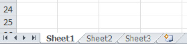
Figure 9–1. Keeping tabs on your sheets: The three default sheets

Click any tab and you'll be taken to that worksheet, which should look just like any other one. As already indicated, all the addresses on the sheets are identical, meaning that their cell references are the same (which raises a question I'll answer in a little while: How exactly does one differentiate between cell S12 on Sheet1 and cell S12 on Sheet2?).

Adding and Moving New Worksheets

To add, or insert, a new sheet into the workbook, you can click the Insert Worksheet button (or use its keyboard equivalent, Shift+F11) to the immediate right of Sheet3 (see Figure 9–2).

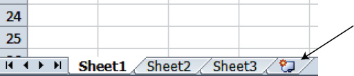
Figure 9–2. The Insert Worksheet button

That click will install another sheet to the right of the existing sheets (to be called Sheet4, etc.). If you right-click a sheet tab, however, you can click Insert on the resulting context menu (see Figure 9–3).

Figure 9–3. Another way to insert a new sheet

That click will call up an Insert dialog box, in which the Worksheet option will be selected by default (see Figure 9–4). Click OK to add the new worksheet.

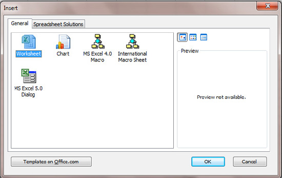
Figure 9–4. An oldie-but-goodie dialog box: That Excel icon dates back a few versions

Note that this sequence isn't exactly equivalent to using the Insert Worksheet button demonstrated earlier, because here the new worksheet will be inserted to the left of whichever worksheet you right-click. Thus, if you right-click and click Insert on Sheet3, the new Sheet4 will appear between Sheet2 and Sheet3, even though it'll be numbered out of sequence.

There's even a third way to insert a new sheet, by clicking the Home Insert Insert Sheet in the Cells button group (see Figure 9–5).

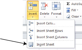
Figure 9–5. Yet another way to insert a new worksheet

Thistoo will insert a new sheet to the left of the sheet tab that's been clicked.

But whatever method you choose, don't worry. If you decide a worksheet tab isn't where you want it to be, you can move it by clicking the tab and dragging it to a new position. As you drag, you'll see a page symbol accompanied by a black down arrow, indicating where the sheet will land when you release the mouse. In Figure 9–6, Sheet3 will be moved between Sheet1 and Sheet2.

Figure 9–6. On the move: Sheet3, en route to a new location

But if you've added many sheets to the workbook, you won't be able to see all the sheet tabs at the same time (see Figure 9–7).

Figure 9–7. Not all there: You can't see sheets 1 through 5

By clicking the arrows shown on the left in Figure 9–8, you can reveal additional sheets in either direction.

Figure 9–8. Exposing hidden sheet tabs by clicking the arrows

The left-pointing arrow accompanied by the vertical bar will, when clicked, reveal the first sheet tab; the right-pointing arrow with the vertical bar will reveal the last tab in your current complement. But these arrow maneuvers don't take you “into” another sheet; they just reveal the sheet tabs. If you're currently working on Sheet10 when you start clicking, you'll stay inside Sheet10.

Deleting Sheets

If you want to delete a sheet, right-click the sheet tab and select the Delete option on the context menu. If the sheet has data on it, the prompt in Figure 9–9 will appear.

Figure 9–9. Note this prompt well—if you click Delete, the data on the sheet will be permanently deleted.

That prompt means business. What it's saying is that if you click Delete, the sheet will be dispatched irrevocably to the digital void—that is, you won't be able to undo the deletion. What you'd have to do, then, if you did delete the sheet in error, is resort to the ancient plan B—just close the workbook without saving it, and then reopen it. That strategy is messy, because you may lose other changes you may have wanted to save, but at least you'll get your sheet back.

Copying a Sheet

You can also copy a sheet in its entirety by right-clicking that sheet tab, clicking Move or Copy…, and clicking Create a copy in the resulting dialog box (see Figure 9–10).

Figure 9–10. Yes, this dialog box gives you another option for moving a sheet, too.

Click the sheet before which you want the copy to appear, and click OK. The copy will then install itself there. If you make a copy of Sheet3, it will be named Sheet3(2). But as you're about to learn, you can rename sheets, too.

Renaming and Recoloring the Worksheet Tabs

You can also rename the worksheet tabs in one of two ways. For one, you can right-click the tab you want to change and click Rename in the context menu. The text appears selected in black, and you just type the new name and press Enter (see Figure 9–11).

Figure 9–11. Once the text is highlighted in black, type a new name and press Enter.

Alternatively, you can double-click the tab. That will likewise select the tab directly, again turning it black. Then type the new name and press Enter.

If you want to recolor a tab, right-click the tab and click Tab Color. You'll see the options shown in Figure 9–12.

Figure 9–12. You've heard of tab collars? These are tab colors.

Just click the color you prefer, and the tab will take on that hue. Keep in mind, though, that when you click the recolored tab, it more or less reverts to its original white color. It's only when you click on a different tab that you'll see the new color you've selected (see Figure 9–13).

Figure 9–13. Changing tab colors

Notice that on the left in Figure 9–13, the Sheet3 tab has been clicked, making it appear mostly white. On the right in the figure, Sheet2 has been clicked, which allows Sheet3's color to appear fully.

Hiding Sheets

You can also easily hide a sheet, and there may be good reasons for wanting to do so, though top-secret confidentiality isn't one of them. For example, you may want to hide a sheet containing complex formulas that other viewers don't need to know about. Also, when you hide a sheet, no one—including you—will be able to accidentally overwrite any of the formulas or inflict any other inadvertent damage. To hide a sheet, just right-click its tab and select Hide. Presto, the sheet disappears.

When you want to restore the sheet to view, just right-click any available sheet tab and click Unhide…, and you'll see the dialog shown in Figure 9–14.

Figure 9–14. Where to get your hidden sheet(s) back

Click the name of the sheet you want to reveal (you can hide more than one), click OK, and it will be back in plain sight.

Grouping Sheets: Changing Multiple Sheets at the Same Time

Excel makes it easy to group several sheets simultaneously, so that changes made to any one sheet will affect the others in the same way; and this option applies both to data entry and formatting.

To get a grasp on what this means, suppose you've designed a workbook, each of whose sheets is devoted to a different employee in a small business. You want every sheet to look the same, with cell A3 containing the caption “Employee Name” in each sheet and A4 displaying the phrase “Social Security Number.” Once you group the sheets, all you have to do is enter these captions on just one sheet—and “Employee Name” will appear in every cell A3, and “Social Security Number” in every A4. That's a very efficient way to work, because your business might have a staff of 50 people—and why should you enter the same things 50 times if you can get away with entering them just once?

By the same token, you might want these captions to exhibit a 24-point font size on all the sheets. Again, by grouping the sheets you need only make that change on one sheet, and the change will be automatically extended to all the others.

How to Group Sheets

There are a few ways to group sheets, and they're all pretty easy. If you want to group all the sheets in your workbook, just right-click any sheet tab and click Select All Sheets (in this context, the word select is identical to group) on the resulting menu. That's it. Your worksheet title will now be accompanied by the word [Group], too, as shown in Figure 9–15.

Figure 9–15. What you'll see alongside your workbook title when you group sheets

When sheets are selected, their tabs turn white (of course, one sheet will always appear white, because you have to always be “in” at least one sheet), as shown in Figure 9–16.

Figure 9–16. Before grouping all the sheets (left) and after (right). The boldfaced text represents the active sheet—the one you're currently working with.

That's the quickest way to group all the sheets in a workbook. If you want to group just some sheets, click the first sheet tab you want to group, and then hold down the Ctrl key and click any other sheet(s). In Figure 9–17, Sheet1 and Sheet3 have been selected. Note that Sheet2 displays the default gray color because it hasn't been selected.

Figure 9–17. Selecting multiple sheets

If you want to group several consecutive sheets, but not all the sheets in your workbook (say, sheets 1 through 5 in an 8-sheet workbook), click the first sheet tab you want to select, and then hold down the Shift key and click the last in the series (in our case Sheet5). All the sheets between 1 and 5 will be selected as well.

One you've carried out the grouping you can start to enter data on the sheet you're currently viewing—and whatever data you entered will appear in the same cells in the other grouped sheets. And the same applies to any formatting changes.

Ungrouping the Sheets

Sooner or later you'll want to ungroup the sheets—because you'll probably need to enter data in a particular sheet that you won't want reproduced in another. For example, once you've entered the “Employee Name” caption in grouped-sheet mode, you'll naturally want to go on and enter specific employee names on specific sheets. But if you don't ungroup the sheets first, the first name you enter will appear on all the sheets. The standard way to ungroup sheets is to right-click any grouped sheet and click Ungroup Sheets on the resulting menu.

Referring to Cells in Other Worksheets: Using Them in Formulas

Worksheets are, as the name suggests, analogous to pages or sheets in a book. But unlike the hard-copy variety, the information contained on these sheets can be referred to and actively used by other sheets in formulas.

For example, you may want to add the salaries of two or more employees in your company, and that information may be stored in different sheets. How then would you go about adding them in one formula?

The problem is, as already indicated, every sheet has the same bundle of 16 billion addresses; so if each salary is placed in cell its respective cell A3, how is each distinguished from the other and utilized in the same formula besides?

This short exercise will show you how:

1. On a blank spreadsheet, type 23000 in cell A3 on Sheet1, and type 32500 in A3 on Sheet2 (don't worry about formatting here).
2. Now, we want to add these two values—let's say in a formula in D5 on Sheet1. Click in D5 and type =, and then, as usual, click cell A3 and type +, as shown in Figure 9–18. So far, we haven't done anything new.
   

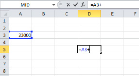
   Figure 9–18. Starting to write the formula on Sheet1. First we use cell A3 from Sheet1.

3. Then click the Sheet2 tab and click cell A3 on that sheet, as shown in Figure 9–19.
   

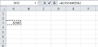
   Figure 9–19. Now Sheet2. Note the formula in the formula bar.

4. Then press Enter, or click the check mark by the formula bar. The result, 55500, appears in D5 of Sheet1—where you wanted it to go. The formula reads

The formula first refers to the value on Sheet1, 23000. We then clicked the other cell whose value we wanted to add, also called A3, but on Sheet2, and that's why we had to click the Sheet2 tab first. In order to distinguish between the two A3s, Excel added the Sheet2! prefix when we clicked that sheet's A3.

That's how Excel works with cells in different sheets—by supplementing cell addresses with the name of the sheet in which the cell is positioned. And if you're asking why the first A3 wasn't preceded by the prefix Sheet1! in our formula, good question. It's because Excel assumes by default that any cells referred to in a formula are on the same sheet as the formula. It's only when a cell is located elsewhere that the prefix is needed.

Using Ranges on Other Sheets in Formulas

Your ability to write formulas and functions that call upon cells in other sheets isn't restricted to individual cells. It's easy to work with whole ranges, too.

Say you have a range of values on Sheet2, C11:C15, whose sum you want to calculate on Sheet1 (see Figure 9–20).

Figure 9–20. Values on Sheet2

1. To start the process, click in the cell on Sheet1 in which you want the answer to appear.
2. Now, because we're working with a range, we could use the SUM function. Let's say you click in cell C12 on Sheet1, where you want the answer to appear. You can then click the AutoSum button, and you'll see what's shown in Figure 9–21.
   

   Figure 9–21. Where's the range between the parentheses?

3. You won't see any cell references yet, because there are no values in the column above C12, nor are there any in the row to C12's left (values that AutoSum is programmed to look for—but that doesn't bother us, because the values we want to add are on Sheet2 anyway). Next, click the Sheet2 tab and simply drag the range you want, as in Figure 9–22.
   

   Figure 9–22. Dragging the range on Sheet2. Again, note how the formula bar records this expression.

4. Then just click OK or click the check mark. On Sheet1, you'll see the answer, as shown in Figure 9–23.

Figure 9–23. The answer, recorded in cell C12 on Sheet1

Again, the range referenced between SUM's parentheses is on Sheet2, and that Sheet2! prefix is Excel's way of declaring that this range is not C11:C15 on Sheet1, in which the function has been written.

Using the View Context Tab to Show and Hide Basic Screen Elements

The Excel worksheet features a number of characteristics that are so basic you probably don't even think about them—namely, the gridlines that demarcate each cell, and the row and column headings that help you identify cell addresses. But if you want, you can remove these elements from the worksheet (though of course you can always return them to the screen when you want).

So why would you want to do this? After all, the cell gridlines and row and column headers help you line up cells visually. The answer to the question, then, is presentational. Once you've completed a worksheet and finished your design work and formula-writing, and you need to show it to others, eliminating the gridlines and headers imparts a cleaner look to your data. Compare the two views shown in Figure 9–24.

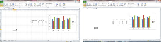
Figure 9–24. The same worksheet, with and without cell gridlines and row and column headers

Turning these elements off and back on is easy. Just click the View tab, and click Gridlines and/or Headings in the Show button group (see Figure 9–25).

Figure 9–25. Show and tell: Where to turn gridlines and headings on and off

Just uncheck the boxes to turn the features off, and check the boxes again to turn the features back on. And as you see, you can even hide the formula bar, too.

Showing Formulas in Cells

If you've constructed a workbook with lots of formulas, you may need to inspect the formulas for mistakes, or at least review them to remind yourself exactly how you put the worksheet together. With that in mind, you can tell Excel to show the formulas in their cells instead of the results of those formulas.

To show the formulas in a particular worksheet's cells, click File Options Advanced, and then check the Show formulas in cells instead of their calculated results box in the Display options for this worksheet area (see Figure 9–26).

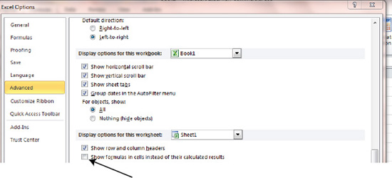
Figure 9–26. Where to display worksheet formulas in their cells

Click OK. All your worksheet's formulas will now appear in their cells, something like Figure 9–27.

Figure 9–27. What you'll see in the cell instead of the result

To turn this visual effect off, return to the Advanced area of the File tab and uncheck the Show formulas in cells instead of their calculated results option.

Hiding the Ribbon

To take matters even further, if you right-click any tab and click Minimize the Ribbon on the ensuing menu, the ribbon will disappear, too (see Figure 9–28). And if you're looking for a keyboard equivalent, try Ctrl-F1.

Figure 9–28. The ribbon—nowhere to be found

Needless to say, you can get the ribbon back by right-clicking the context tab heading and deselecting Minimize the Ribbon (see Figure 9–29), or executing Ctrl-F1 a second time.

Figure 9–29. Getting your ribbon back

A related option is Full Screen, found in the Workbook Views button group within the View context tab (see Figure 9–30).

Figure 9–30. The Workbook Views button group

Click it and your screen will change to look like Figure 9–31.

Figure 9–31. Nothing but screen: The Full Screen view

To get the normal view back, just press the Esc key, or click the standard Restore button in the upper-right corner of the window(the middle of the three buttons you'll see there), or double-click the worksheet's Title Bar – the border at the very uppermost part of the screen bearing the workbook's title..

Keeping Important Data in View with the Freeze Panes Option

There may be times when you'll be working with a lengthy worksheet database containing many rows and/or columns, and you want to keep the header row—and/or column—in view.

For example, say you've devised a worksheet that compiles sales data for salespersons by week, across a series of columns—52 to be exact, spanning an entire year (see Figure 9–32).

Figure 9–32. A weekly sales data worksheet

The problem—a classic spreadsheet dilemma—is that once you begin scrolling to the right in order to view the later weeks, the first columns disappear (see Figure 9–33).

Figure 9–33. The salesperson names and weeks 1 through 3 are no longer visible.

The solution is to click the Freeze Panes button in the Window button group on the View tab (see Figure 9–34).

Figure 9–34. The Freeze Panes button

In order to ensure that the salesperson names persist on the screen no matter how far to the right you scroll, click anywhere in the workbook (as long as you can see column A) and click Freeze Panes Freeze First Column. That will draw a black line down the boundary between columns A and B (see Figure 9–35).

Figure 9–35. The black line tells you that the first column (A) will be remain in view even when you scroll to the right.

Now if you scroll right, you'll see what's shown in Figure 9–36.

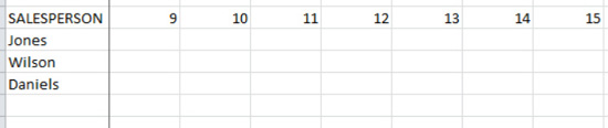
Figure 9–36. Can't stay away: The salesperson names are still there

And you can do the same for the first row, by clicking Freeze Top Row.

To turn off a freeze view, click Freeze Panes Unfreeze Panes.

Freezing Rows and Columns at the Same Time

There may be other times when you need to freeze some rows and columns simultaneously. In our case, we might want to always be able to see both the salesperson names and the week numbers as we scroll in either direction—vertically or horizontally. Thus, we'd want to freeze the salesperson name column and the row listing week numbers, something like Figure 9–37.

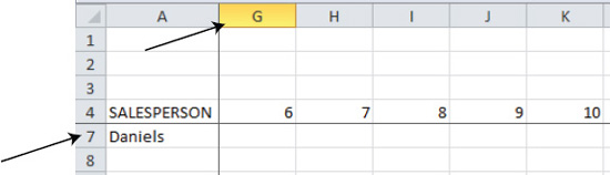
Figure 9–37. The first two salesperson names and the first five week numbers have disappeared, because we've scrolled both down and across the worksheet after having clicked Freeze Panes. Note the row header numbers and column header gaps (4 through 7 and A through G).

To achieve this effect, you need to click the Freeze Panes option once you decide exactly which rows and columns you want to freeze. The rule is this: to freeze a column you click in the column immediately to the right of the one you want to freeze, and to freeze a row you click in the row immediately beneath the one you want to freeze. Thus, in this case you'd click in the cell shown in Figure 9–38.

Figure 9–38. Clicking directly to the right of the column you want to freeze and directly beneath the row you want to freeze

Once you've gotten a handle on where you want to locate the freeze, click Freeze Panes Freeze Panes. If you've discovered you've clicked in the wrong place, just click the Unfreeze Panes option and try again.

Protecting the Worksheet and the Workbook

Once you've put all that work into your workbook, having outfitted it with rows of complex formulas and breathtaking charts, you may get a bit nervous about what might happen next. What if you were to accidentally overwrite—or delete—a formula? True, you might be able to bring it back with an Undo command, but that prospect would depend on exactly when you discovered the mishap. Worse yet, what if your five-year-old nephew began to type some formulas of his own on the sheet?

Have no fear. Excel has anticipated those calamities, by allowing you to protect your workbooks and individual worksheets with a set of options that should help you fend off little Timmy's editorial changes and leave your masterpiece intact.

By way of introduction, you need to understand what protecting a sheet does and doesn't do. Protecting a sheet won't seal off your sheet with industrial-strength invincibility, foiling the bad guys who want to compromise or steal your data. Not quite, because workbook and worksheet protection is more about warding off mistakes than disarming hackers who have your formulas in their sights. Still, protection can do a pretty good job of, well, protecting your work.

The process of protecting worksheets and workbooks is actually quite easy, but the details get a bit quirky, as you'll see.

Protecting a Worksheet

To start the process of protecting a worksheet (you can try this out on a blank worksheet), just click anywhere in the sheet, click the Review tab, and select Protect Sheet from the Changes button group (see Figure 9–39).

Figure 9–39. The Changes button group. We want to click Protect Sheet here, not Protect Workbook.

When you click Protect Sheet, you'll see the dialog shown in Figure 9–40.

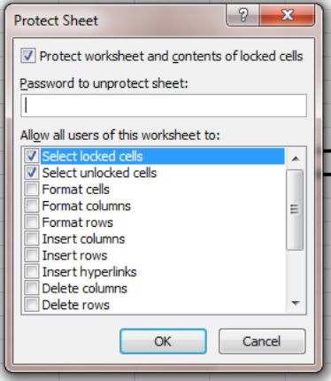
Figure 9–40. The Protect Sheet dialog box

Note that some check boxes are selected by default, and typically you'll accept these and simply click OK. The various options displayed in the dialog box give you control over exactly which operations you'll allow a user to perform on various worksheet elements (e.g., whether a user will be allowed to format cells or insert rows even if the worksheet is protected). If you accept all the defaults and click OK, the worksheet won't look any different. But when you try to type anything in any cell, you'll be greeted with the prompt shown in Figure 9–41 even before you can press Enter.

Figure 9–41. Do not enter: What you'll see when you try to enter data in a cell in a protected worksheet

You'll be prevented from entering the data, and that's what protecting a worksheet largely entails—blocking any subsequent data entry to a worksheet.

Again, you should understand the limitations of worksheet protection. Even though users will be prevented from entering data on the protected sheet, no one will be stopped from copying the data on that sheet and pasting it into another workbook.

Using a Password: Some Extra Protection

You also can devise an optional password you'll be asked to enter in order to protect the sheet. When you first choose a password, another dialog box will then ask you to retype or confirm it (see Figure 9–42).

Figure 9–42. How to enter a sheet protection password

Unprotecting a Worksheet

Needless to say, once you've protected the worksheet, you may decide you need to return the sheet to its original unprotected state so that it can receive data entries again. All you have to do is go back to the Changes button group, where you'll see that the Protect Sheet button has toggled to display Unprotect Sheet (see Figure 9–43).

Figure 9–43. Flip side: The Unprotect Sheet button is the same one you clicked to protect the sheet

Just click Unprotect Sheet, and the sheet will be unprotected again—type away.

If you've used a password to protect a sheet and later decide to unprotect it, clicking Unprotect Sheet willcall up an Unprotect Sheet dialog box, prompting you to reenter your password, as shown in Figure 9–44.

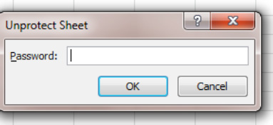
Figure 9–44. The Unprotect Sheet dialog box requests your password if you've selected one.

Just make sure you've written that password down somewhere, because if you forget it, you won't be able to unprotect the sheet. Remember as well that if you haven't availed yourself of the password possibility, anyone else can unprotect the worksheet—provided of course they know how to do that.

Protecting Some, but Not All, of a Worksheet

In some cases, you may want to be able to enter data in some cells in a worksheet, even as the remainder of the cells are blocked or protected. Recall our grading worksheet, in which we calculated point bonus awards that supplemented students' test scores (see Chapter 4). In such a case, you might want to protect the cells containing the bonus formulas while continuing to leave other cells available, in which you could enter additional student test scores.

So how do you protect some, but not all, of a worksheet? It's here where some of those workbook protection quirks mentioned earlier come into play.

In order to make some cells available to receive data in a worksheet that's otherwise protected, you need first to select those cells and instruct Excel not to protect them.

The following short exercise will demonstrate how this works:

1. Select cells B7:B16.
2. Now click Home Format Format Cells… in the Cells button group, as shown in Figure 9–45.
   

   Figure 9–45. Starting the individual cell protection process by clicking Format Cells….

3. After selecting that option, you'll be reintroduced to an old friend, the Format Cells dialog box; only this time, you need to click one of its tabs that we haven't visited before: Protection (see Figure 9–46).
   

   Figure 9–46. The Protection tab of the Format Cells dialog box

4. Note that the Locked check box is checked by default. That means simply that if you protect the sheet, all its cells will be protected. But since you've selected B7:B16, uncheck the Locked box. Now, once you protect the sheet, cells B7:B16 will still remain unlocked—that is, you'll be able to enter data in only these cells.

And that's how unlocking cells works—first you designate those cells to be unlocked, and only then do you protect the sheet. So now if you activate workbook protection, it will still be possible to enter data in cells B7:B16.

Hiding Formulas

Earlier in this chapter I described how you can reveal your worksheet's formulas in the cells in which they're written. There's also a kind of flip side to this option—you can hide worksheet formulas so that they can't be seen at all, not even in the formula bar.

To hide formulas in cells, you have to work prospectively and select those cells before you protect the worksheet, just as when unlocking selected cells. The following exercise demonstrates:

1. Enter these values shown in Figure 9–47 in cells D4:D8 and perform a SUM in cell D9.
   

   Figure 9–47. Note the formula bar

2. Then return to the Format Cells dialog box and click the Protection tab (see Figure 9–48).
   

   Figure 9–48. The Format Cells dialog box. Note the caption beneath the Hidden option.

3. Click Hidden, and then click OK. Then protect the worksheet, and click in cell D9 and observe the formula bar (see Figure 9–49).

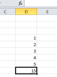
Figure 9–49. Drawing a blank: The formula's no longer visible

The formula is nowhere to be seen, even though it's still safely stored in cell D9. To restore the formula to view, just unprotect the sheet.

Protecting a Workbook

You can also protect an entire workbook, which does something completely different from protecting a worksheet.

When you protect a workbook, you protect what Excel calls its structure—and that means that when workbook protection is turned on, you won't be able to delete or move a worksheet, or restore a hidden worksheet to view.

Another workbook protection option—a less central one—enables you to protect the window arrangement of worksheets. If, for example, you resize a worksheet window and you need to maintain precisely that worksheet size and position on the screen, protecting the workbook for windows will hold the worksheet right there—and you'll be able neither to move nor resize it (see Figure 9–50).

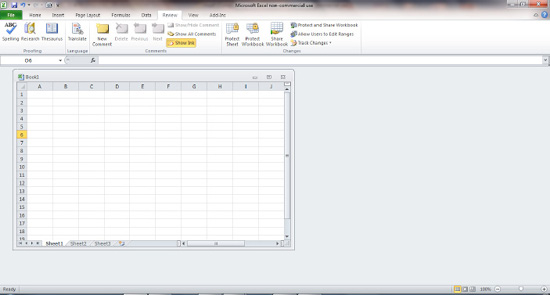
Figure 9–50 . A downsized worksheet

To protect a workbook, click the Review tab, and click Protect Workbook in the Changes button group (see Figure 9–51).

Figure 9–51. Protecting a workbook

You'll next see the dialog shown in Figure 9–52.

Figure 9–52. Note that the dialog box isn't titled Protect Workbook, but that's what it's about to do.

Note again that you're provided with a password option. Whether you use a password or not, when you click OK you won't be able to move, delete, or add any worksheet—but you will continue to be able to enter and edit data and formulas.

Unprotecting a Workbook

Unprotecting a workbook is about as easy as it gets. Just click the Protect Workbook button a second time. Oddly enough, unlike the Protect Sheet button, the Protect Workbook button doesn't appear as “Unprotect Workbook” once you've protected the workbook. It just doesn't change. Of course, if you've designated a password, you'll be prompted to supply it before you can unprotect the workbook.

Summary

Every Excel workbook gives its users a massive amount of territory to work with, and knowing how to work with its multisheet character is a valuable asset. Next, we'll explore what you need to know to print your Excel data once you decide to commit all the information you've compiled in a workbook to hard copy.