Contents
Introduction
Most choice experiments involve conducting a market research survey. The survey consists of a series of questions about attributes of interest about a potential new product or product modification. For example, a computer manufacturer might be interested in manufacturing a new laptop and wants information about customer preference before beginning an expensive development process. Computer characteristics change so rapidly that it is crucial to quickly identify the attributes that help the manufacturers to design and build a new machine most likely to capture enough market share to be profitable.
Often, the attributes are obvious. For example, the consumer wants a laptop that has a large screen, weighs almost nothing, costs almost nothing, and lasts forever on a single battery charge. The question, then, is how much is the customer willing to compromise these desires? How important is each of these attributes, and which kinds of trade off is the customer most likely to accept and still purchase a new machine?
Assume a simple situation where a computer manufacturer wants to examine preferences for four possible laptop configurations. Notice that there are no ‘right’ or ‘wrong’ selections. Instead there are just preferences. A well designed questionnaire and proper analysis of results can tell a manufacturer how to proceed. The manufacturer wants information about the following four laptop attributes.
• size of hard drive disk (40 GB or 80 GB)
• speed of processor (1.5 GHz or 2.0 GHz)
• battery life (4 Hrs or 6 Hrs)
• cost of computer ($1000, $1200 or $1500)
If a survey were constructed that offered the possibility of choosing any combination of these attributes, a respondent would be forced to evaluate 24 possible combinations and make a single response. Instead each respondent usually evaluates several choice sets and for each choice set, chooses the preferred profile. In the simplest situation, each respondent chooses between sets of two profiles.
Then, you analyze the choices of multiple respondents. A well designed choice experiment, correctly analyzed is a efficient way to give the researcher the most information for the least time and expense.
Table 1 shows hypothetical results from a single survey designed to collect information about consumer preferences about laptop computers.
• Each column in the survey identifies a laptop attribute.
• Each line in the survey defines a laptop profile, which is a collection of attribute values.
• Each choice set consists of two attribute profiles.
• All of the attribute values are allowed to change across the two profiles in a choice set.
|
For each pair, please check the combination of attributes you find most appealing.
|
||||||
|
|
|
Disk Size
|
Speed
|
Battery Life
|
Price
|
Preference
|
|
1
|
1
|
40 GB
|
1.5 GHz
|
6 hours
|
$1,000
|
_X_
|
|
|
2
|
80 GB
|
1.5 GHz
|
4 hours
|
$1,200
|
___
|
|
|
|
|
|
|
|
|
|
2
|
1
|
40 GB
|
1.5 GHz
|
4 hours
|
$1,500
|
___
|
|
|
2
|
80 GB
|
2.0 GHz
|
4 hours
|
$1,200
|
_X_
|
|
|
|
|
|
|
|
|
|
3
|
1
|
40 GB
|
2.0 GHz
|
4 hours
|
$1,200
|
_X_
|
|
|
2
|
80 GB
|
2.0 GHz
|
6 hours
|
$1,500
|
___
|
|
|
|
|
|
|
|
|
|
4
|
1
|
40 GB
|
2.0 GHz
|
4 hours
|
$1,000
|
_X_
|
|
|
2
|
80 GB
|
1.5 GHz
|
6 hours
|
$1,200
|
___
|
|
|
|
|
|
|
|
|
|
5
|
1
|
40 GB
|
1.5 GHz
|
6 hours
|
$1,000
|
_X_
|
|
|
2
|
40 GB
|
2.0 GHz
|
4 hours
|
$1,500
|
___
|
|
|
|
|
|
|
|
|
|
6
|
1
|
40 GB
|
2.0 GHz
|
6 hours
|
$1,200
|
_X_
|
|
|
2
|
80 GB
|
1.5 GHz
|
4 hours
|
$1,500
|
___
|
|
|
|
|
|
|
|
|
|
7
|
1
|
40 GB
|
2.0 GHz
|
6 hours
|
$1,500
|
___
|
|
|
2
|
80 GB
|
1.5 GHz
|
4 hours
|
$1,000
|
_X_
|
|
|
|
|
|
|
|
|
|
8
|
1
|
40 GB
|
1.5 GHz
|
4 hours
|
$1,200
|
___
|
|
|
2
|
80 GB
|
2.0 GHz
|
4 hours
|
$1,000
|
_X_
|
The DOE Choice designer can create a survey like that shown in Table 9.1. However, to create an effective design, the Choice designer needs information about the attributes. For example, most laptop attributes have values that are intrinsic preferences. That is, a bigger disk size is better, longer battery life is better, and so forth. The purpose of conducting a choice survey is to find out how potential laptop purchasers feel about the advantages of a collection of attributes.
One way to gain prior information about attributes in a survey is to conduct a single example survey, analyze the results, and use those results as prior information to create the final survey instrument.
This chapter shows how to create a sample survey and use its results as prior information for a final survey design.
Create an Example Choice Experiment
The Choice design can create a survey like the one in Table 1.
1. Choose DOE > Choice Design, and complete the initial dialog as shown in Figure 9.1.
Figure 9.1 Choice Design Dialog with Attributes Defined

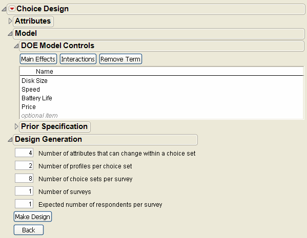
2. Click Continue. For this example, use the default values in the Model Control panel and in the Design Generation panel, as shown in Figure 9.2.
Optionally, you can use the DOE Model Controls panel to add interactions to the choice model in situations where you expect there are interactions and want to generate profile sets that will help detect them.
Figure 9.2 Design Generation Panel for the Laptop Experiment

The values in the Design Generation panel describe the laptop survey.
Number of attributes that can change within a choice set
There are four laptop attributes. Entering 4 as the number of attributes that can change within a choice set means that the Choice designer can change 4 or fewer attribute values within a single choice set. You can enter fewer than the total number of attributes to constrain the total number that can be changed within a choice set. This might be a reasonable thing to do if you had a large number of attributes and you want to make it easier for the respondents to make a choice. For example, a survey might be interested in 20 or more attributes of a cell phone, but show and change only 5 or fewer attributes in a choice set.
Number of profiles per choice set
This example has two profiles per choice set. You can design choice experiments with more than two profiles in a choice set.
Number of choice sets per survey
There are eight choice sets in the example survey but often there are many more.
Number of surveys
The example only shows a single survey. Normally you expect multiple respondents and would request more than one survey.
Expected number of respondents per survey
You might want to give surveys to 10 people, but use two different surveys. So you enter 2 as the Number of surveys and 5 as the Expected number of respondents per survey.
Note: Recall that this first example is used to generate prior information, then used to create a more realistic survey. This example is a single survey given to a single respondent.
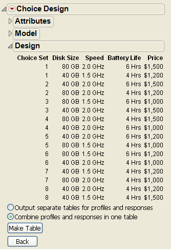
3. Click Make Design to see the example survey results in Figure 9.3.
Figure 9.3 Survey Results based on a Simple Model and Default Prior Information

The Radio buttons beneath the design settings let you choose between having the survey settings in one JMP table and gathering survey results in a second table, or generating a single table that shows the settings and has an additional column for the choice response.
You can see that there are eight choice sets, each consisting of two laptop profiles. At this point you can press Back and modify the design, or click Make Table and generate the JMP table shown in Figure 9.4.
This default design was created with no given prior information. Without prior information, the Choice designer has no way of knowing which attribute levels are better. That is, the Choice designer cannot know that a lower price might be more desirable than a higher price, a faster machine is better than a slower machine, and so forth. As a result, you can see that some choice sets might not convey useful information. The analysis results are used as prior information in a new Choice design dialog.
Figure 9.4 JMP Data Table for Preliminary Laptop Choice Survey

Analyze the Example Choice Experiment
Once a survey design is complete, a respondent chooses one profile from each set, entering ‘1’ for the chosen profile and ‘0’ for the rejected profile. Suppose a respondent completed the example survey as shown in Figure 9.5. You can now analyze these results using the Choice platform in the Analyze menu (Analyze > Modeling > Choice).
Figure 9.5 JMP Table with Survey Choice Sets and Responses

1. Click the Choice script in the Laptop Design data table and select Run Script to analyze that data with the Choice modeling platform from the Analyze menu.
When you run the Choice model script, the Choice launch dialog shown in Figure 9.6 appears. The Choice dialog is designed to cover a variety of choice survey results, which can include data saved in multiple data tables. This example has all data contained in a single table. For details about using the Choice analysis dialog, see the Choice Modeling chapter in the Modeling and Multivariate Methods book.
Figure 9.6 Choice Model Fitting Dialog

2. Click Run Model on the Choice model fitting dialog.
3. An additional dialog then appears asking if this is a one-table analysis with all the data in the Profile Table, which is the case in this sample survey. Click Yes in this dialog to continue.
The analysis shows as in Figure 9.7.
To design the final choice survey using prior information, you will need to enter estimates of the mean and variance of the attribute parameter estimates. The analysis on the left in Figure 9.7 has estimates of the attribute means, called Estimate, and estimates of the standard deviation of the attributes, called Std Error. An easy way to see the variance of the attributes is to capture the analysis in a JMP table and compute the variance:
4. Right click on the Parameter Estimates report and choose Make into Data Table from the menu, as shown.
5. In the new Untitled data table, create a new column and call it Var.
6. Select Formula from the Cols menu (Cols > Formula), or right-click at the top of the Var column and select Formula for the menu that shows.
7. In the Formula Editor, click the Std Error column in the column list and click the exponent button ( ) on the formula editor panel to compute the variance shown on the right in Figure 9.7.
Figure 9.7 Analysis of the sample Laptop Survey

This preliminary survey with its analysis gives you the information needed to design a final survey appropriate for gathering information from multiple respondents. Keep in mind that in a real situation, you might have prior information about factor attributes and not need to do a sample design.
Note: Leave the Untitled data table with the mean and variance information open to be used in the next example.
Design a Choice Experiment Using Prior Information
In some situations, you will know from previous surveys or experience how to give prior information to the Choice designer about product attributes. This example continues by designing the laptop experiment again, using the analysis information gained from the sample design.
1. Choose DOE > Choice Design and enter the attributes and values as before.
2. Click Continue to see the Choice design panels in Figure 9.8.
3. Now enter the values from the JMP table created by the previous analysis into the Prior Mean and Prior Variance Matrix panels of the Choice Design dialog, as shown in Figure 9.8. You can copy-and-paste to transfer the values from the data table to the Choice dialog panels.
Figure 9.8 Enter Prior Mean and Variance Information from Preliminary Survey

4. Enter the values into the Design Generation panel, as shown in Figure 9.9.
– Four or fewer attribute levels can change within a choice set.
– There are two profiles per choice set.
– Each survey has eight choice sets.
– The design generates two separate surveys.
– Five respondents are expected to complete each survey (for a total of 10 respondents).
Figure 9.9 Design Specifications for final Laptop Survey

5. Click Make Design. A partial view of the design is shown in Figure 9.10.
Figure 9.10 Design Runs for Two Choice Surveys

6. Click Make Table. The final data table will have runs for ten survey respondents, giving a total of 160 observations (2 profiles * 8 choice sets * 2 surveys * 5 respondents = 160 observations).
Administer the Survey and Analyze Results
The survey data table with its results is stored in the Sample Data Design Experiment folder installed with JMP. Figure 9.11 is a partial listing of the survey data table with results. The Choice script created by the Choice designer and saved with the survey data table can be used to analyze the data. The default data table created by the Choice designer is named Choice Profiles. Note in Figure 9.11, the data table name is changed to Laptop Results.
Initial Choice Platform Analysis
1. To continue the example, open the table called Laptop Results.jmp, saved in the Sample Data folder.
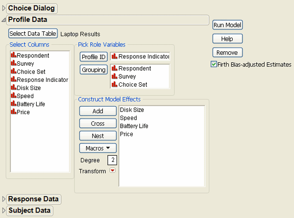
2. To analyze the data, click the Choice script saved with the data and select Run Script from the menu to see the completed dialog shown in Figure 9.11.
Note that this dialog has three grouping variables (Respondent, Survey, and Choice Set, whereas the dialog shown Figure 9.6 had only the Choice Set grouping variable because there was a single survey and a single respondent. This example included multiple surveys and respondents, which must be included in the analysis.
Figure 9.11 Choice Model Fitting Dialog to Analyze the Laptop Survey

3. Click Run Model on the Fit Model dialog. The query again appears asking if the analysis is a one-table analysis with all the data in the profile table. Click Yes to see the initial analysis result shown in Figure 9.12.
The results are clear. While all the effects are significant, the most significant attribute is Speed.
Figure 9.12 Initial Analysis of the Final Laptop Survey

Find Unit Cost and Trade Off Costs with the Profiler
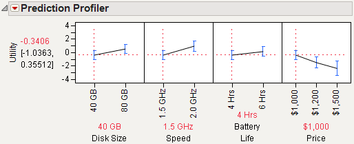
You would like to know how changing the price, or other characteristics, of a laptop affects the desirability as perceived by potential buyers. This desirability is called the utility value of the laptop attributes. The profiler shows the utility value and how it changes as the laptop attributes change.
1. Select Profiler from the menu on the Choice Model title bar to see the Prediction Profiler in Figure 9.13.
Figure 9.13 Default Prediction Profiler for Laptop Choice Analysis

When each attribute value is set to its lowest value, the Utility value is –0.3406. The first thing you want to know is the unit utility cost.
2. To find the unit utility cost, move the trace for Price to $1,500 and note how the Utility value changes.
Compare the Utility values in Figure 9.13 and Figure 9.14. The value of Utility changes from –0.3406 to –2.3303 when cost is raised from $1,000 to $1,500. That is, raising the price of a laptop $500.00 lowers the utility (or desirability) approximately 2 units. Thus, you can say that the unit utility cost is roughly $250.00.
Figure 9.14 Compare Change in Utility Over Price

With this unit utility cost estimate you can now vary the other attributes, note the change in utility, and find an approximate dollar value associated with that attribute change. For example, the most significant attribute is speed (see Figure 9.12).
3. In the Prediction Profiler, set Price to its lowest value and change Speed to its higher value.
You can see in Figure 9.15 that the Utility value changes from the original value shown in Figure 9.13 of –0.3406 to 0.9886, for a total change of 1.3292 units. If the unit utility cost is estimated to be $250.00, as shown above, then the increase in price for a 2.0 GHz laptop over a 1.5 GHz laptop can be computed to be 1.3292*$250.00 = $332.30. This is the dollar value the Choice survey provides the manufacturer as a basis for pricing different laptop products. You can make similar calculations for the other attributes.
Figure 9.15 Change Speed in Profiler and Note Utility Value

This simple Choice survey and its analysis shows how this kind if information can be used to help manufacturers and retailers identify important product attributes and assign values to them.
The Choice designer allows more complex designs, such as designs with interactions and other terms. The Choice analysis platform can be used to analyze complex designs, and it can be used to incorporate data from multiple data sets that include demographic information about the respondents.
..................Content has been hidden....................
You can't read the all page of ebook, please click here login for view all page.
