
Contents
Examples of Nonlinear Designs
The Nonlinear Designer allows scientists to generate optimal designs and optimally augment data for fitting models that are nonlinear in their parameters. Such models, when they are descriptive of the underlying process, can yield more accurate prediction of process behavior than is possible with the standard polynomial models.
To use the Nonlinear Designer, you first need a data table that has
• one column for each factor
• one column for the response
• a column that contains a formula showing the functional relationship between the factor(s) and the response.
This is the same format for a table you would supply to the nonlinear platform for modeling.
The first example in this section describes how to approach creating a nonlinear design when there is prior data. The second example describes how to approach creating the design without data, but with reasonable starting values for the parameter estimates.
Using Nonlinear Fit to Find Prior Parameter Estimates
Suppose you have already collected experimental data and placed it in a JMP data table. That table can be used to create a nonlinear design for improving the estimates of the model’s parameters.
To follow along with this example, open Chemical Kinetics.jmp from the Nonlinear Examples folder found in the sample data installed with JMP.
Chemical Kinetics.jmp (Figure 12.1) contains a column (Model (x))whose values are formed by a formula with a poor guess of the parameter values.
Figure 12.1 Chemical Kinetics.jmp

First, fit the data to the model using nonlinear least squares to get better parameter values.
1. Select Analyze > Modeling > Nonlinear.
2. Select Velocity (y) and click Y, Response on the nonlinear launch dialog.
3. Select Model (x) and click X, Predictor Formula (see Figure 12.2). Note that the formula given by Model (X) shows in the launch dialog.
Figure 12.2 Initial Nonlinear Analysis Launch Dialog

4. Click OK on the launch dialog to see the Nonlinear control panel.
5. Click the Go button on the Nonlinear control panel to see the results (Figure 12.3).
The Save Estimates button adds the new fitted parameter values in the Model (x) column in the Chemical Kinetics.jmp data table.
The Confidence Limits button computes confidence intervals used to create a nonlinear design.
The ranges for LowerCL and UpperCL are the intervals for Vmax and k. They are asymptotically normal. Use these limits to create a nonlinear design in JMP.
Figure 12.3 Nonlinear Fit Results

6. Click the Confidence Limits button to produce confidence intervals.
7. Click Save Estimates to add the new fitted parameter values in the Model (x) column in the Chemical Kinetics.jmp data table.
The Model (x) column properties show the new parameter estimates.
Figure 12.4 New Parameter Estimates

Note: Leave the nonlinear analysis report open because these results are needed in the DOE nonlinear design dialog described next.
Now create a design for fitting the model’s nonlinear parameters.
1. With the Chemical Kinetics.jmp data table open, select DOE > Nonlinear Design.
2. Complete the launch dialog the same way as the Nonlinear Analysis launch dialog shown previously. That is, Select Velocity (y) and click Y, Response. Select Model (x) and click the X, Predictor Formula. Figure 12.5 shows the completed dialog.
Figure 12.5 Initial Nonlinear Design Launch Dialog

3. Click OK to see the completed Design panels for factors and parameters, as shown in Figure 12.6.
Figure 12.6 Nonlinear Design Panels for Factors and Parameters

Note that in Chemical Kinetics.jmp (Figure 12.1), the range of data for Concentration goes from 0.417 to 6.25. Therefore, these values initially appear as the high and low values in the Factors control panel as follows:
4. Change the factor range for Concentration to a broader interval—from 0.1 to 7 (Figure 12.7).
Note that the a priori distribution of the parameters Vmax and k is Normal, which is correct for this example. Change the current level of uncertainty in the two parameters using the analysis results.
5. Look back at the analysis report in Figure 12.3 and locate the upper and lower confidence limits for Vmax and k in the Solution table. Change the values for Vmax and k to correspond to those limits, as shown in Figure 12.7.
Now you have described the current level of uncertainty of the two parameters.
Figure 12.7 Change Values for Factor and Parameters
6. If necessary, type the desired number of runs (17 is the default value for this example) into the text box.
Use commands from the menu on the Nonlinear Design title bar to get the best possible design:
7. Select Number of Starts from the menu on the title bar and enter 100 in the text box.
8. Select Advanced Options > Number of Monte Carlo Samples and enter 2 in the text box.
9. Click Make Design to preview the design (Figure 12.8). Your results might differ from those shown for the additional runs.
Figure 12.8 Selecting the Number of Runs

10. Click Make Table.
This creates a new JMP design table (Figure 12.9) whose rows are the runs defined by the nonlinear design.
Note: This example creates a new table to avoid altering the sample data table Chemical Kinetics.jmp. In most cases, however, you can augment the original table using the Augment Table option in the Nonlinear Designer instead of making a new table. This option adds the new runs shown in the Design to the existing data table.
Figure 12.9 Making a Table with the Nonlinear Designer

The new runs use the wider interval of allowed concentration, which leads to more precise estimates of k and Vmax.
Creating a Nonlinear Design with No Prior Data
This next example describes how to create a design when you have not yet collected data, but have a guess for the unknown parameters.
To follow along with this example, open Reaction Kinetics Start.jmp, found in the Design Experiment folder in the sample data installed with JMP. Notice that the table is a template. That is, the table has columns with properties and formulas, but there are no observations in the table. The design has not yet been created and data have not been collected.
This table is used to supply the formula in the yield model column to the Nonlinear DOE platform. The formula is used to create a nonlinear design for fitting the model’s nonlinear parameters.
Figure 12.10 Yield Model Formula

This model is from Box and Draper (1987). The formula arises from the fractional yield of the intermediate product in a consecutive chemical reaction. It is written as a function of time and temperature.
1. With the Reaction Kinetics Start.jmp data table open, select DOE > Nonlinear Design to see the initial launch dialog.
2. Select observed yield and click Y, Response.
3. Select yield model (the column with the formula) and click X, Predictor Formula.
The completed dialog should look like the one in Figure 12.11.
Figure 12.11 Nonlinear Design launch Dialog

4. Click OK to see the nonlinear design Factors and Parameters panels in Figure 12.12.
5. Change the two factors’ values to be a reasonable range of values. (In your experiment, these values might have to be an educated guess.) For this example, use the values 510 and 540 for Reaction Temperature. Use the values 0.1 and 0.3 for Reaction Time.
6. Change the values of the parameter t1 to 25 and 50, and t3 to 30 and 35.
7. Click on the Distribution of each parameter and select Uniform from the menu to change the distribution from the default Normal (see Figure 12.12).
8. Change the number of runs to 12 in the Design Generation panel.
Figure 12.12 Change Factor Values, Parameter Distributions, and Number of Runs
9. Click Make Design, then Make Table. Your results should look similar to those in Figure 12.13.
Figure 12.13 Design Table
10. To analyze data that contains values for the response, observed yield, open Reaction Kinetics.jmp from the Design Experiment folder in the sample data installed with JMP (Figure 12.14).
Figure 12.14 Reaction Kinetics.jmp

First, examine the design region with an overlay plot.
11. Select Graph > Overlay Plot.
12. Remove all existing column assignments.
13. Select Reaction Temperature and click Y
14. Select Reaction Time and click X as shown in the Overlay Plot launch dialog in Figure 12.15.
15. Click OK to see the overlay plot in Figure 12.15.
Figure 12.15 Create an Overlay Plot

Notice that the points are not at the corners of the design region. In particular, there are no points at low temperature and high time—the lower right corner of the graph.
16. Select Analyze > Modeling > Nonlinear.
17. Remove all existing column assignments.
18. Select observed yield and click Y, Response.
19. Select yield model and click the X, Predictor Formula, then click OK.
20. Click Go on the Nonlinear control panel.
21. Now, choose Profilers > Profiler from the red triangle menu on the Nonlinear Fit title bar.
22. To maximize the yield, choose Maximize Desirability from the red triangle menu on the Prediction Profiler title bar.
The maximum yield is approximately 63.5% at a reaction temperature of 540 degrees Kelvin and a reaction time of 0.1945 minutes.
Figure 12.16 Time and Temperature Settings for Maximum Yield

Creating a Nonlinear Design
To begin, open a data table that has a column whose values are formed by a formula (for details about formulas, see the Using JMP). This formula must have parameters.
Select DOE >Nonlinear Design, or click the Nonlinear Design button on the JMP Starter DOE page. Then, follow the steps below:
Identify the Response and Factor Column with Formula
1. Open a data table that contains a column whose values are formed by a formula that has parameters. This example uses Corn.jmp from the Nonlinear Examples folder in the sample data installed with JMP.
2. Select DOE > Nonlinear Design to see the initial launch dialog.
3. Select yield and click Y, Response. The response column cannot have missing values.
4. Select quad and click X, Predictor Formula. The quad variable has a formula that includes nitrate and three parameters (Figure 12.17).
5. Click OK on the launch dialog to see the Nonlinear Design DOE panels.
Figure 12.17 Identify Response (Y) and the Column with the Nonlinear Formula (X)
Set Up Factors and Parameters in the Nonlinear Design Dialog
First, look at the formula for quad, shown in Figure 12.18, and notice there are three parameters. These parameters show in the Parameters panel of the Nonlinear design dialog, with initial parameter values.
Figure 12.18 Formula for quad has Parameters a, b, and c

Use Figure 12.19 to understand how to set up factor and parameter names and values.
• The initial values for the factor and the parameters are reasonable and do not need to be changed.
• If necessary, change the Distribution of the parameters to Uniform, as shown in Figure 12.19.
Figure 12.19 Example of Setting Up Factors and Parameters

Enter the Number of Runs and Preview the Design
1. The Design Generation panel shows 150 as the default number of runs. This number includes observations in the current data. 147 runs are desired. Since there are originally 144 rows, 3 additional runs need to be added. Enter 147 in the Number of Runs edit box.
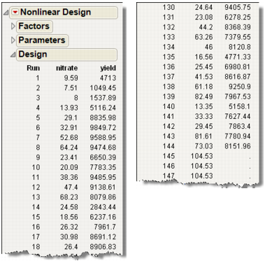
2. Click Make Design before creating the data table to preview the design. Figure 12.20 shows a partial listing of the design.
Figure 12.20 Example Preview Design
Make Table or Augment the Table
3. The last step is to click either Make Table or Augment Table. The Make Table command creates a new table (Figure 12.21) with all runs included. The Augment Table command adds the new runs to the existing table.
Figure 12.21 Partial Listing of an Example Nonlinear Design Table
Advanced Options for the Nonlinear Designer
For advanced users, the Nonlinear Designer has the two additional options, as shown in Figure 12.22. These advanced options are included because finding nonlinear DOE solutions involves minimizing the integral of the log of the determinant of the Fisher information matrix with respect to the prior distribution of the parameters. These integrals are complicated and have to be calculated numerically.
The way the integration is done for Normal distribution priors uses a numerical integration technique where the integral is reparameterized into a radial direction, and the number of parameters minus one angular directions. The radial part of the integral is handled using Radau-Gauss-Laguerre quadrature with an evaluation at radius=0. A randomized Mysovskikh quadrature is used to calculate the integral over the spherical part, which is equivalent to integrating over the surface of a hypersphere.
Note: If some of the prior distributions are not Normal, then the integral is reparameterized so that the new parameters have normal distribution, and then the radial-spherical integration method is applied. However, if the prior distribution set for the parameters does not lend itself to a solution, sometimes the process fails and gives the message that the Fisher information is singular in a region of the parameter space, and advises changing the prior distribution or the ranges of the parameters.
Figure 12.22 Advanced Options for the Nonlinear Designer

The following is a technical description for these two advanced options:
Number of Monte Carlo Samples
sets the number of octahedra per sphere. Because each octahedron is a fixed unit, this option can be thought of as setting the number of octahedra per sphere.
N Monte Carlo Spheres
are the number of nonzero radius values used. The default is two spheres and one center point. Each radial value requires integration over the angular dimensions. This is done by constructing a certain number of hyperoctahedra (the generalization of an octagon in arbitrary dimensions), and randomly rotating each of them.
Technical The reason for the approach given by these advanced options is to get good integral approximations much faster than using standard methods. For instance, with six parameters, using two radii and one sample per sphere, these methods give a generalized five- point rule that needs only 113 observations to get a good approximation. Using the most common approach (Simpson’s rule) would need 56 = 15,625 evaluations. The straight Monte Carlo approach also requires thousands of function evaluations to get the same level of quality in the answer. For more details, see Gotwalt, Jones, and Steinberg (2009).
Keep in mind that if the number of radii is set to zero, then just the center point is used, which gives a local design that is optimal for a particular value of the parameters. For some people this is good enough for their purposes. These designs are created much faster than if the integration is performed.
..................Content has been hidden....................
You can't read the all page of ebook, please click here login for view all page.