
Contents
Launching the Sample Size and Power Platform
The Sample Size and Power platform helps you plan your study for a single mean or proportion comparison, a two sample mean or proportion comparison, a one-sample standard deviation comparison, a k sample means comparison, or a counts per unit comparison. Depending upon your experimental situation, you supply one or two quantities to obtain a third quantity. These quantities include:
• required sample size
• expected power
• expected effect size
When you select DOE > Sample Size and Power, the panel in Figure 16.1 appears with button selections for experimental situations. The following sections describe each of these selections and explain how to enter the quantities and obtain the desired computation.
Figure 16.1 Sample Size and Power Choices

One-Sample and Two-Sample Means
After you click either One Sample Mean, or Two Sample Means in the initial Sample Size selection list (Figure 16.1), a Sample Size and Power window appears. (See Figure 16.2.)
Figure 16.2 Initial Sample Size and Power Windows for Single Mean (left) and Two Means (right)

The windows are the same except that the One Mean window has a button at the bottom that accesses an animation script.
The initial Sample Size and Power window requires values for Alpha, Std Dev (the error standard deviation), and one or two of the other three values: Difference to detect, Sample Size, and Power. The Sample Size and Power platform calculates the missing item. If there are two unspecified fields, a plot is constructed, showing the relationship between these two values:
• power as a function of sample size, given specific effect size
• power as a function of effect size, given a sample size
• effect size as a function of sample size, for a given power.
The Sample Size and Power window asks for these values:
Alpha
s the probability of a type I error, which is the probability of rejecting the null hypothesis when it is true. It is commonly referred to as the significance level of the test. The default alpha level is 0.05. This implies a willingness to accept (if the true difference between groups is zero) that, 5% (alpha) of the time, a significant difference is incorrectly declared.
Std Dev
is the error standard deviation. It is a measure of the unexplained random variation around the mean. Even though the true error is not known, the power calculations are an exercise in probability that calculates what might happen if the true value is the one you specify. An estimate of the error standard deviation could be the root mean square error (RMSE) from a previous model fit.
Extra Parameters
is only for multi-factor designs. Leave this field zero in simple cases. In a multi-factor balanced design, in addition to fitting the means described in the situation, there are other factors with extra parameters that can be specified here. For example, in a three-factor two-level design with all three two-factor interactions, the number of extra parameters is five. (This includes two parameters for the extra main effects, and three parameters for the interactions.) In practice, the particular values entered are not that important, unless the experimental range has very few degrees of freedom for error.
Difference to Detect
is the smallest detectable difference (how small a difference you want to be able to declare statistically significant) to test against. For single sample problems this is the difference between the hypothesized value and the true value.
Sample Size
is the total number of observations (runs, experimental units, or samples) in your experiment. Sample size is not the number per group, but the total over all groups.
Power
is the probability of rejecting the null hypothesis when it is false. A large power value is better, but the cost is a higher sample size.
Continue
evaluates at the entered values.
Back
returns to the previous Sample Size and Power window so that you can either redo an analysis or start a new analysis.
Animation Script
runs a JSL script that displays an interactive plot showing power or sample size. See the section, Sample Size and Power Animation for One Mean, for an illustration of the animation script.
Single-Sample Mean
Using the Sample Size and Power window, you can test if one mean is different from the hypothesized value.
For the one sample mean, the hypothesis supported is
and the two-sided alternative is
where μ is the population mean and μ0 is the null mean to test against or is the difference to detect. It is assumed that the population of interest is normally distributed and the true mean is zero. Note that the power for this setting is the same as for the power when the null hypothesis is H0: μ=0 and the true mean is μ0.
Suppose you are interested in testing the flammability of a new fabric being developed by your company. Previous testing indicates that the standard deviation for burn times of this fabric is 2 seconds. The goal is to detect a difference of 1.5 seconds when alpha is equal to 0.05, the sample size is 20, and the standard deviation is 2 seconds. For this example, μ0 is equal to 1.5. To calculate the power:
1. Select DOE > Sample Size and Power.
2. Click the One Sample Mean button in the Sample Size and Power Window.
3. Leave Alpha as 0.05.
4. Leave Extra Parameters as 0.
5. Enter 2 for Std Dev.
6. Enter 1.5 as Difference to detect.
7. Enter 20 for Sample Size.
8. Leave Power blank. (See the left window in Figure 16.3.)
9. Click Continue.
The power is calculated as 0.8888478174 and is rounded to 0.89. (See right window in Figure 16.3.) The conclusion is that your experiment has an 89% chance of detecting a significant difference in the burn time, given that your significance level is 0.05, the difference to detect is 1.5 seconds, and the sample size is 20.
Figure 16.3 A One-Sample Example

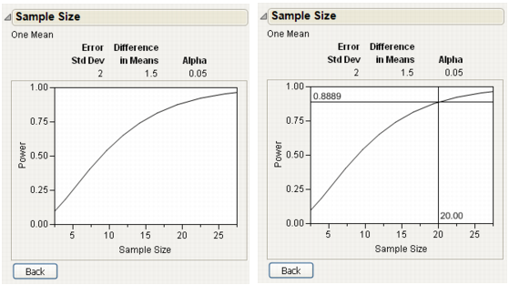
Power versus Sample Size Plot
To see a plot of the relationship of Sample Size and Power, leave both Sample Size and Power empty in the window and click Continue.
The plots in Figure 16.4, show a range of sample sizes for which the power varies from about 0.1 to about 0.95. The plot on the right in Figure 16.4 shows using the crosshair tool to illustrate the example in Figure 16.3.
Figure 16.4 A One-Sample Example Plot
Power versus Difference Plot
When only Sample Size is specified (Figure 16.5) and Difference to Detect and Power are empty, a plot of Power by Difference appears, after clicking Continue.
Figure 16.5 Plot of Power by Difference to Detect for a Given Sample Size

Sample Size and Power Animation for One Mean
Clicking the Animation Script button on the Sample Size and Power window for one mean shows an interactive plot. This plot illustrates the effect that changing the sample size has on power. As an example of using the Animation Script:
1. Select DOE > Sample Size and Power.
2. Click the One Sample Mean button in the Sample Size and Power Window.
3. Enter 2 for Std Dev.
4. Enter 1.5 as Difference to detect.
5. Enter 20 for Sample Size.
6. Leave Power blank.
The Sample Size and Power window appears as shown on the left of Figure 16.6.
7. Click Animation Script.
The initial animation plot shows two t-density curves. The red curve shows the t-distribution when the true mean is zero. The blue curve shows the t-distribution when the true mean is 1.5, which is the difference to be detected. The probability of committing a type II error (not detecting a difference when there is a difference) is shaded blue on this plot. (This probability is often represented as β in the literature.) Similarly, the probability of committing a type I error (deciding that the difference to detect is significant when there is no difference) is shaded as the red areas under the red curve. (The red-shaded areas under the curve are represented as α in the literature.)
Select and drag the square handles to see the changes in statistics based on the positions of the curves. To change the values of Sample Size and Alpha, click on their values beneath the plot.
Figure 16.6 Example of Animation Script to Illustrate Power

Two-Sample Means
The Sample Size and Power windows work similarly for one and two sample means; the Difference to Detect is the difference between two means. The comparison is between two random samples instead of one sample and a hypothesized mean.
For testing the difference between two means, the hypothesis supported is
and the two-sided alternative is
where μ1 and μ2 are the two population means and D0 is the difference in the two means or the difference to detect. It is assumed that the populations of interest are normally distributed and the true difference is zero. Note that the power for this setting is the same as for the power when the null hypothesis is and the true difference is D0.
Suppose the standard deviation is 2 (as before) for both groups, the desired detectable difference between the two means is 1.5, and the sample size is 30 (15 per group). To estimate the power for this example:
1. Select DOE > Sample Size and Power.
2. Click the Two Sample Means button in the Sample Size and Power Window.
3. Leave Alpha as 0.05.
4. Enter 2 for Std Dev.
5. Leave Extra Parameters as 0.
6. Enter 1.5 as Difference to detect.
7. Enter 30 for Sample Size.
8. Leave Power blank.
9. Click Continue.
The Power is calculated as 0.51. (See the left window in Figure 16.7.) This means that you have a 51% chance of detecting a significant difference between the two sample means when your significance level is 0.05, the difference to detect is 1.5, and each sample size is 15.
Plot of Power by Sample Size
To have a greater power requires a larger sample. To find out how large, leave both Sample Size and Power blank for this same example and click Continue. Figure 16.7 shows the resulting plot, with the crosshair tool estimating that a sample size of about 78 is needed to obtain a power of 0.9.
Figure 16.7 Plot of Power by Sample Size to Detect for a Given Difference

k-Sample Means
Using the k-Sample Means option, you can compare up to 10 means. Consider a situation where 4 levels of means are expected to be in the range of 10 to 13, the standard deviation is 0.9, and your sample size is 16.
The hypothesis to be tested is:
H0: μ1=μ2=μ3=μ4 versus Ha: at least one mean is different
To determine the power:
1. Select DOE > Sample Size and Power.
2. Click the k Sample Means button in the Sample Size and Power Window.
3. Leave Alpha as 0.05.
4. Enter 0.9 for Std Dev.
5. Leave Extra Parameters as 0.
6. Enter 10, 11, 12, and 13 as the four levels of means.
7. Enter 16 for Sample Size.
8. Leave Power blank.
9. Click Continue.
The Power is calculated as 0.95. (See the left of Figure 16.8.) This means that there is a 95% chance of detecting that at least one of the means is different when the significance level is 0.05, the population means are 10, 11, 12, and 13, and the total sample size is 16.
If both Sample Size and Power are left blank for this example, the sample size and power calculations produce the Power versus Sample Size curve. (See the right of Figure 16.8.) This confirms that a sample size of 16 looks acceptable.
Notice that the difference in means is 2.236, calculated as square root of the sum of squared deviations from the grand mean. In this case it is the square root of (–1.5)2+ (–0.5)2+(0.5)2+(1.5)2, which is the square root of 5.
Figure 16.8 Prospective Power for k-Means and Plot of Power by Sample Size

One Sample Standard Deviation
Use the One-Sample Standard Deviation option on the Sample Size and Power window (Figure 16.1) to determine the sample size needed for detecting a change in the standard deviation of your data. The usual purpose of this option is to compute a large enough sample size to guarantee that the risk of a type II error, β, is small. (This is the probability of failing to reject the null hypothesis when it is false.)
In the Sample Size and Power window, specify:
Alpha
is the significance level, usually 0.05. This implies a willingness to accept (if the true difference between standard deviation and the hypothesized standard deviation is zero) that a significant difference is incorrectly declared 5% of the time.
Hypothesized Standard Deviation
is the hypothesized or baseline standard deviation to which the sample standard deviation is compared.
Alternative Standard Deviation
can select Larger or Smaller from the menu to indicate the direction of the change you want to detect.
Difference to Detect
is the smallest detectable difference (how small a difference you want to be able to declare statistically significant). For single sample problems this is the difference between the hypothesized value and the true value.
Sample Size
is how many experimental units (runs, or samples) are involved in the experiment.
Power
is the probability of declaring a significant result. It is the probability of rejecting the null hypothesis when it is false.
In the lower part of the window you enter two of the items and the Sample Size and Power calculation determines the third.
Some examples in this chapter use engineering examples from the online manual of The National Institute of Standards and Technology (NIST). You can access the NIST manual examples at http://www.itl.nist.gov/div898/handbook.
One Sample Standard Deviation Example
One example from the NIST manual states a problem in terms of the variance and difference to detect. The variance for resistivity measurements on a lot of silicon wafers is claimed to be 100 ohm-cm. The buyer is unwilling to accept a shipment if the variance is greater than 155 ohm-cm for a particular lot (55 ohm-cm above the baseline of 100 ohm-cm).
In the Sample Size and Power window, the One Sample Standard Deviation computations use the standard deviation instead of the variance. The hypothesis to be tested is:
H0: σ = σ0, where σ0 is the hypothesized standard deviation. The true standard deviation is σ0 plus the difference to detect.
In this example the hypothesized standard deviation, σ0, is 10 (the square root of 100) and σ is 12.4499 (the square root of 100 + 55 = 155). The difference to detect is 12.4499 – 10 = 2.4499.
You want to detect an increase in the standard deviation of 2.4499 for a standard deviation of 10, with an alpha of 0.05 and a power of 0.99. To determine the necessary sample size:
1. Select DOE > Sample Size and Power.
2. Click the One Sample Standard Deviation button in the Sample Size and Power Window.
3. Leave Alpha as 0.05.
4. Enter 10 for Hypothesized Standard Deviation.
5. Select Larger for Alternate Standard Deviation.
6. Enter 2.4499 as Difference to Detect.
7. Enter 0.99 for Power.
8. Leave Sample Size blank. (See the left of Figure 16.9.)
9. Click Continue.
The Sample Size is calculated as 171. (See the right of Figure 16.9.) This result is the sample size rounded up to the next whole number.
Note: Sometimes you want to detect a change to a smaller standard deviation. If you select Smaller from the Alternative Standard Deviation menu, enter a negative amount in the Difference to Detect field.
Figure 16.9 Window To Compare Single-Direction One-Sample Standard Deviation

One-Sample and Two-Sample Proportions
The Sample Size windows and computations to test sample sizes and power for proportions are similar to those for testing means. You enter a true Proportion and choose an Alpha level. Then, for the one-sample proportion case, enter the Sample Size and Null Proportion to obtain the Power. Or, enter the Power and Null Proportion to obtain the Sample Size. Similarly, to obtain a value for Null Proportion, enter values for Sample Size and Power. For the two-sample proportion case, either the two sample sizes or the desired Power must be entered. (See Figure 16.10 and Figure 16.11.)
The sampling distribution for proportions is approximately normal, but the computations to determine sample size and test proportions use exact methods based on the binomial distribution. Exact methods are more reliable since using the normal approximation to the binomial can provide erroneous results when small samples or proportions are used. Exact power calculations are used in conjunction with a modified Wald test statistic described in Agresti and Coull (1998).
The results also include the actual test size. This is the actual Type I error rate for a given situation. This is important since the binomial distribution is discrete, and the actual test size can be significantly different from the stated Alpha level for small samples or small proportions.
One Sample Proportion
Clicking the One Sample Proportion option on the Sample Size and Power window yields a One Proportion window. In this window, you can specify the alpha level and the true proportion. The sample size, power, or the hypothesized proportion is calculated. If you supply two of these quantities, the third is computed, or if you enter any one of the quantities, you see a plot of the other two.
For example, if you have a hypothesized proportion of defects, you can use the One Sample Proportion window to estimate a large enough sample size to guarantee that the risk of accepting a false hypothesis (β) is small. That is, you want to detect, with reasonable certainty, a difference in the proportion of defects.
For the one sample proportion, the hypothesis supported is
and the two-sided alternative is
where p is the population proportion and p0 is the null proportion to test against. Note that if you are interested in testing whether the population proportion is greater than or less than the null proportion, you use a one-sided test. The one-sided alternative is either
or
One-Sample Proportion Window Specifications
In the top portion of the Sample Size window, you can specify or enter values for:
Alpha
is the significance level of your test. The default value is 0.05.
Proportion
is the true proportion, which could be known or hypothesized. The default value is 0.1.
One-Sided or Two-Sided
Specify either a one-sided or a two-sided test. The default setting is the two-sided test.
In the bottom portion of the window, enter two of the following quantities to see the third, or a single quantity to see a plot of the other two.
Null Proportion
is the proportion to test against (p0) or is left blank for computation. The default value is 0.2.
Sample Size
is the sample size, or is left blank for computation. If Sample Size is left blank, then values for Proportion and Null Proportion must be different.
Power
is the desired power, or is left blank for computation.
One-Sample Proportion Example
As an example, suppose that an assembly line has a historical proportion of defects equal to 0.1, and you want to know the power to detect that the proportion is different from 0.2, given an alpha level of 0.05 and a sample size of 100.
1. Select DOE > Sample Size and Power.
2. Click One Sample Proportion.
3. Leave Alpha as 0.05.
4. Leave 0.1 as the value for Proportion.
5. Accept the default option of Two-Sided. (A one-sided test is selected if you are interested in testing if the proportion is either greater than or less than the Null Proportion.)
6. Leave 0.2 as the value for Null Proportion.
7. Enter 100 as the Sample Size.
8. Click Continue.
The Power is calculated and is shown as approximately 0.7 (see Figure 16.10). Note the Actual Test Size is 0.0467, which is slightly less than the desired 0.05.
Figure 16.10 Power and Sample Window for One-Sample Proportions
Two Sample Proportions
The Two Sample Proportions option computes the power or sample sizes needed to detect the difference between two proportions, p1 and p2.
For the two sample proportion, the hypothesis supported is
and the two-sided alternative is
where p1 and p2 are the population proportions from two populations, and D0 is the hypothesized difference in proportions.
The one-sided alternative is either
or
Two Sample Proportion Window Specifications
Specifications for the Two Sample Proportions window include:
Alpha
is the significance level of your test. The default value is 0.05.
Proportion 1
is the proportion for population 1, which could be known or hypothesized. The default value is 0.5.
Proportion 2
is the proportion for population 2, which could be known or hypothesized. The default value is 0.1.
One-Sided or Two-Sided
Specify either a one-sided or a two-sided test. The default setting is the two-sided test.
Null Difference in Proportion
is the proportion difference (D0) to test against, or is left blank for computation. The default value is 0.2.
Sample Size 1
is the sample size for population 1, or is left blank for computation.
Sample Size 2
is the sample size for population 2, or is left blank for computation.
Power
is the desired power, or is left blank for computation.
If you enter any two of the following three quantities, the third quantity is computed:
• Null Difference in Proportion
• Sample Size 1 and Sample Size 2
• Power
Example of Determining Sample Sizes with a Two-Sided Test
As an example, suppose you are responsible for two silicon wafer assembly lines. Based on the knowledge from many runs, one of the assembly lines has a defect rate of 8%; the other line has a defect rate of 6%. You want to know the sample size necessary to have 80% power to reject the null hypothesis of equal proportions of defects for each line.
To estimate the necessary sample sizes for this example:
1. Select DOE > Sample Size and Power.
2. Click Two Sample Proportions.
3. Accept the default value of Alpha as 0.05.
4. Enter 0.08 for Proportion 1.
5. Enter 0.06 for Proportion 2.
6. Accept the default option of Two-Sided.
7. Enter 0.0 for Null Difference in Proportion.
8. Enter 0.8 for Power.
9. Leave Sample Size 1 and Sample Size 2 blank.
10. Click Continue.
The Sample Size window shows sample sizes of 2554. (see Figure 16.11.) Testing for a one-sided test is conducted similarly. Simply select the One-Sided option.
Figure 16.11 Difference Between Two Proportions for a Two-Sided Test

Example of Determining Power with Two Sample Proportions Using a One-Sided Test
Suppose you want to compare the effectiveness of a two chemical additives. The standard additive is known to be 50% effective in preventing cracking in the final product. The new additive is assumed to be 60% effective. You plan on conducting a study, randomly assigning parts to the two groups. You have 800 parts available to participate in the study (400 parts for each additive). Your objective is to determine the power of your test, given a null difference in proportions of 0.01 and an alpha level of 0.05. Because you are interested in testing that the difference in proportions is greater than 0.01, you use a one-sided test.
1. Select DOE > Sample Size and Power.
2. Click Two Sample Proportions.
3. Accept the default value of Alpha as 0.05.
4. Enter 0.6 for Proportion 1.
5. Enter 0.5 for Proportion 2.
6. Select One-Sided.
7. Enter 0.01 as the Null Difference in Proportion.
8. Enter 400 for Sample Size 1.
9. Enter 400 for Sample Size 2.
10. Leave Power blank.
11. Click Continue.
Figure 16.12 shows the Two Proportions windows with the estimated Power calculation of 0.82.
Figure 16.12 Difference Between Two Proportions for a One-Sided Test

You conclude that there is about an 82% chance of rejecting the null hypothesis at the 0.05 level of significance, given that the sample sizes for the two groups are each 400. Note the Actual Test Size is 0.0513, which is slightly larger than the stated 0.05.
Counts per Unit
You can use the Counts per Unit option from the Sample Size and Power window (Figure 16.1) to calculate the sample size needed when you measure more than one defect per unit. A unit can be an area and the counts can be fractions or large numbers.
Although the number of defects observed in an area of a given size is often assumed to have a Poisson distribution, it is understood that the area and count are large enough to support a normal approximation.
Questions of interest are:
• Is the defect density within prescribed limits?
• Is the defect density greater than or less than a prescribed limit?
In the Counts per Unit window, options include:
Alpha
is the significance level of your test. The default value is 0.05.
Baseline Count per Unit
is the number of targeted defects per unit. The default value is 0.1.
Difference to detect
is the smallest detectable difference to test against and is specified in defects per unit, or is left blank for computation.
Sample Size
is the sample size, or is left blank for computation.
Power
is the desired power, or is left blank for computation.
In the Counts per Unit window, enter Alpha and the Baseline Count per Unit. Then enter two of the remaining fields to see the calculation of the third. The test is for a one-sided (one-tailed) change. Enter the Difference to Detect in terms of the Baseline Count per Unit (defects per unit). The computed sample size is expressed as the number of units, rounded to the next whole number.
Counts per Unit Example
As an example, consider a wafer manufacturing process with a target of 4 defects per wafer. You want to verify that a new process meets that target within a difference of 1 defect per wafer with a significance level of 0.05. In the Counts per Unit window:
1. Leave Alpha as 0.05 (the chance of failing the test if the new process is as good as the target).
2. Enter 4 as the Baseline Counts per Unit, indicating the target of 4 defects per wafer.
3. Enter 1 as the Difference to detect.
4. Enter a power of 0.9, which is the chance of detecting a change larger than 1 (5 defects per wafer). In this type of situation, alpha is sometimes called the producer’s risk and beta is called the consumer’s risk.
5. Click Continue to see the results in Figure 16.13, showing a computed sample size of 38 (rounded to the next whole number).
The process meets the target if there are less than 190 defects (5 defects per wafer in a sample of 38 wafers).
Figure 16.13 Window For Counts Per Unit Example

Sigma Quality Level
The Sigma Quality Level feature is a simple statistic that puts a given defect rate on a “six-sigma” scale. For example, on a scale of one million opportunities, 3.397 defects result in a six-sigma process. The computation that gives the Sigma Quality Level statistic is
Sigma Quality Level = NormalQuantile(1 – defects/opportunities) + 1.5
Two of three quantities can be entered to determine the Sigma Quality Level statistic in the Sample Size and Power window:
• Number of Defects
• Number of Opportunities
• Sigma Quality Level
When you click Continue, the sigma quality calculator computes the missing quantity.
Sigma Quality Level Example
As an example, use the Sample Size and Power feature to compute the Sigma Quality Level for 50 defects in 1,000,000 opportunities:
1. Select DOE > Sample Size and Power.
2. Click the Sigma Quality Level button.
3. Enter 50 for the Number of Defects.
4. Enter 1000000 as the Number of Opportunities. (See window to the left in Figure 16.14.)
5. Click Continue.
The results are a Sigma Quality Level of 5.39. (See right window in Figure 16.14.)
Figure 16.14 Sigma Quality Level Example 1

Number of Defects Computation Example
If you want to know how many defects reduce the Sigma Quality Level to “six-sigma” for 1,000,000 opportunities:
1. Select DOE > Sample Size and Power.
2. Click the Sigma Quality Level button.
3. Enter 6 as Sigma Quality Level.
4. Enter 1000000 as the Number of Opportunities. (See left window in Figure 16.14.)
5. Leave Number of Defects blank.
6. Click Continue.
The computation shows that the Number of Defects cannot be more than approximately 3.4. (See right window in Figure 16.15.)
Figure 16.15 Sigma Quality Level Example 2

Reliability Test Plan and Demonstration
You can compute required sample sizes for reliability tests and reliability demonstrations using the Reliability Test Plan and Reliability Demonstration features.
Reliability Test Plan
The Reliability Test Plan feature computes required sample sizes, censor times, or precision, for estimating failure times and failure probabilities.
To launch the Reliability Test Plan calculator, select DOE > Sample Size and Power, and then select Reliability Test Plan. Figure 16.16 shows the Reliability Test Plan window.
Figure 16.16 Reliability Test Plan Window
The Reliability Test Plan window has the following options:
Alpha
is the significance level. It is also 1 minus the confidence level.
Distribution
is the assumed failure distribution, with the associated parameters.
Precision Measure
is the precision measure. In the following definitions, U and L correspond to the upper and lower confidence limits of the quantity being estimated (either a time or failure probability), and T corresponds to the true time or probability for the specified distribution.
Interval Ratio is sqrt(U/L), the square root of the ratio of the upper and lower limits.
Two-sided Interval Absolute Width is U-L, the difference of the upper and lower limits.
Lower One-sided Interval Absolute Width is T-L, the true value minus the lower limit.
Two-sided Interval Relative Width is (U-L)/T, the difference between the upper and lower limits, divided by the true value.
Lower One-sided Interval Relative Width is (T-L)/T, the difference between the true value and the lower limit, divided by the true value.
Objective
is the objective of the study. The objective can be one of the following two:
– estimate the time associated with a specific probability of failure.
– estimate the probability of failure at a specific time.
CDF Plot
is a plot of the CDF of the specified distribution. When estimating a time, the true time associated with the specified probability is written on the plot. When estimating a failure probability, the true probability associated with the specified time is written on the plot.
Sample Size
is the required number of units to include in the reliability test.
Censor Time
is the amount of time to run the reliability test.
Precision
is the level of precision. This value corresponds to the Precision Measure chosen above.
Large-sample approximate covariance matrix
gives the approximate variances and covariance for the location and scale parameters of the distribution.
Continue
click here to make the calculations.
Back
click here to go back to the Power and Sample Size window.
After the Continue button is clicked, two additional statistics are shown:
Expected number of failures
is the expected number of failures for the specified reliability test.
Probability of fewer than 3 failures
is the probability that the specified reliability test will result in fewer than three failures. This is important because a minimum of three failures is required to reliably estimate the parameters of the failure distribution. With only one or two failures, the estimates are unstable. If this probability is large, you risk not being able to achieve enough failures to reliably estimate the distribution parameters, and you should consider changing the test plan. Increasing the sample size or censor time are two ways of lowering the probability of fewer than three failures.
Example
A company has developed a new product and wants to know the required sample size to estimate the time till 20% of units fail, with a two-sided absolute precision of 200 hours. In other words, when a confidence interval is created for the estimated time, the difference between the upper and lower limits needs to be approximately 200 hours. The company can run the experiment for 2500 hours. Additionally, from studies done on similar products, they believe the failure distribution to be approximately Weibull (2000, 3).
To compute the required sample size, do the following steps:
1. Select DOE > Sample Size and Power.
2. Select Reliability Test Plan.
3. Select Weibull from the Distribution list.
4. Enter 2000 for the Weibull α parameter.
5. Enter 3 for the Weibull β parameter.
6. Select Two-sided Interval Absolute Width from the Precision Measure list.
7. Select Estimate time associated with specified failure probability.
8. Enter 0.2 for p.
9. Enter 2500 for Censor Time.
10. Enter 200 for Precision.
11. Click Continue. Figure 16.17 shows the results.
Figure 16.17 Reliability Test Plan Results
The required sample size is 217 units if the company wants to estimate the time till 20% failures with a precision of 200 hours. The probability of fewer than 3 failures is small, so the experiment will likely result in enough failures to reliably estimate the distribution parameters.
Reliability Demonstration
A reliability demonstration consists of testing a specified number of units for a specified period of time. If fewer than k units fail, you pass the demonstration, and conclude that the product reliability meets or exceeds a reliability standard.
The Reliability Demonstration feature computes required sample sizes and experimental run-times for demonstrating that a product meets or exceeds a specified reliability standard.
To launch the Reliability Demonstration calculator, select DOE > Sample Size and Power, and then select Reliability Demonstration. Figure 16.18 shows the Reliability Demonstration window.
Figure 16.18 Reliability Demonstration Window

The Reliability Demonstration window has the following options:
Alpha
is the alpha level.
Distribution
is the assumed failure distribution. After selecting a distribution, specify the associated scale parameter in the text field under the Distribution menu.
Max Failures Tolerated
is the maximum number of failures you want to allow during the demonstration. If we observe this many failures or fewer, then we say we passed the demonstration.
Time
is the time component of the reliability standard you want to meet.
Probability of Surviving
is the probability component of the reliability standard you want to meet.
Time of Demonstration
is the required time for the demonstration.
Number of Units Tested
is the required number of units for the demonstration.
Continue
click here to make the calculations.
Back
click here to go back to the Power and Sample Size window.
After the Continue button is clicked, a plot appears (see Figure 16.19).
Figure 16.19 Reliability Demonstration Plot

The true probability of a unit surviving to the specified time is unknown. The Y axis of the plot gives the probability of passing the demonstration (concluding the true reliability meets or exceeds the standard) as a function of the true probability of a unit surviving to the standard time. Notice the line is increasing, meaning that the further the truth is above the standard, the more likely you are to detect the difference.
Example
A company wants to get the required sample size for assessing the reliability of a new product against an historical reliability standard of 90% survival after 1000 hours. From prior studies on similar products, it is believed that the failure distribution is Weibull, with a β parameter of 3. The company can afford to run the demonstration for 800 hours, and wants the experiment to result in no more than 2 failures.
To compute the required sample size, do the following steps:
1. Select DOE > Sample Size and Power.
2. Select Reliability Demonstration.
3. Select Weibull from the Distribution list.
4. Enter 3 for the Weibull β.
5. Enter 2 for Max Failures Tolerated.
6. Enter 1000 for Time.
7. Enter 0.9 for Probability of Surviving.
8. Enter 800 for Time of Demonstration.
9. Click Continue. Figure 16.20 shows the results.
Figure 16.20 Reliability Demonstration Results
The company needs to run 118 units in the demonstration. Furthermore, if they observe 2 or fewer failures by 800 hours, we can conclude that the new product reliability is at least as reliable as the standard.
..................Content has been hidden....................
You can't read the all page of ebook, please click here login for view all page.