
Contents
Creating Screening Experiments
You can use the screening designer in JMP to create screening designs, but the custom designer is more flexible and general. The straightforward screening examples described below show that ‘custom’ does not mean ‘exotic.’ The custom designer is a general purpose design environment that can create screening designs.
Creating a Main-Effects-Only Screening Design
To create a main-effects-only screening design using the custom designer:
1. Select DOE > Custom Design.
2. Enter six continuous factors into the Factors panel (see Step 1: Design the Experiment, for details). Figure 3.2 shows the six factors.
3. Click Continue. The default model contains only the main effects.
4. Using the default of 12 runs, click Make Design. Click the disclosure button ( on Windows and
  on the Macintosh) to open the Design Evaluation outline node.
Note: The result is a resolution-three screening design. All the main effects are estimable, but they are confounded with two factor interactions.
Figure 3.2 A Main-Effects-Only Screening Design

5. Click the disclosure buttons beside Design Evaluation and then beside Alias Matrix ( on Windows and
  on the Macintosh) to open the Alias Matrix. Figure 3.3 shows the Alias Matrix, which is a table of zeros, ones, and negative ones.
The Alias Matrix shows how the coefficients of the constant and main effect terms in the model are biased by any active two-factor interaction effects not already added to the model. The column labels identify interactions. For example, for the X1 row, the columns labeled X2*X4 and X2*X5 have 0.333. This means that the expected value of the main effect of X1 is actually the sum of the main effect of X1 plus 0.333 times the effect of X2*X4, plus 0.333 times the effect of X2*X5, and so on for the rest of the X1 row. You are assuming that these interactions are negligible in size compared to the effect of X1.
Figure 3.3 The Alias Matrix

Note to DOE experts: The Alias matrix is a generalization of the confounding pattern in fractional factorial designs.
Creating a Screening Design to Fit All Two-Factor Interactions
There is risk involved in designs for main effects only. The risk is that two-factor interactions, if they are strong, can confuse the results of such experiments. To avoid this risk, you can create experiments resolving all the two-factor interactions.
Note to DOE experts: The result in this example is a resolution-five screening design. Two-factor interactions are estimable but are confounded with three-factor interactions.
1. Select DOE > Custom Design.
2. Enter five continuous factors into the Factors panel (see Step 1: Design the Experiment in Introduction to Designing Experiments for details).
3. Click Continue.
4. In the Model panel, select Interactions > 2nd.
5. In the Design Generation Panel choose Minimum for Number of Runs and click Make Design.
Figure 3.4 shows the runs of the two-factor design with all interactions. The sample size, 16 (a power of two) is large enough to fit all the terms in the model. The values in your table may be different from those shown below.
Figure 3.4 All Two-Factor Interactions

6. Click the disclosure button ( on Windows and
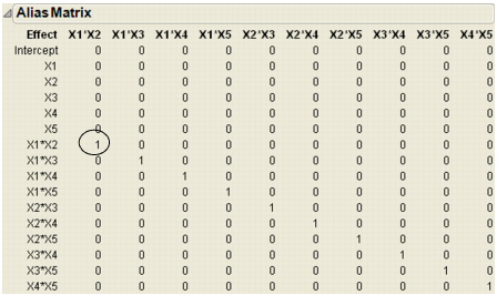
  on the Macintosh) and to open the Design Evaluation outlines, then open Alias Matrix. Figure 3.5 shows the alias matrix table of zeros and ones. The columns labels identify an interaction. For example, the column labelled X1*X2 refers to the interaction of the first and second effect, the column labelled X2*X3 refers to the interaction between the second and third effect, and so forth.
Look at the column labelled X1*X2. There is only one value of 1 in that column. All others are 0. The 1 occurs in the row labelled X1*X2. All the other rows and columns are similar. This means that the expected value of the two-factor interaction X1*X2 is not biased by any other terms. All the rows above the row labelled X1*X2 contain only zeros, which means that the Intercept and main effect terms are not biased by any two-factor interactions.
Figure 3.5 Alias Matrix Showing all Two-Factor Interactions Clear of all Main Effects
A Compromise Design Between Main Effects Only and All Interactions
In a screening situation, suppose there are six continuous factors and resources for n = 16 runs. The first example in this section showed an eight-run design that fit all the main effects. With six factors, there are 15 possible two-factor interactions. The minimum number of runs that could fit the constant, six main effects and 15 two-factor interactions is 22. This is more than the resource budget of 16 runs. It would be good to find a compromise between the main-effects only design and a design capable of fitting all the two-factor interactions.
This example shows how to obtain such a design compromise using the custom designer.
1. Select DOE > Custom Design.
2. Define six continuous factors (X1 - X6).
3. Click Continue. The model includes the main effect terms by default. The default estimability of these terms is Necessary.
4. Click the Interactions button and choose 2nd to add all the two-factor interactions.
5. Select all the interaction terms and click the current estimability (Necessary) to reveal a menu. Change Necessary to If Possible.
6. Type 16 in the User Specified edit box in the Number of Runs section, as shown. Although the desired number of runs (16) is less than the total number of model terms, the custom designer builds a design to estimate as many two-factor interactions as possible.
7. Click Make Design.
After the custom designer creates the design, click the disclosure button beside Design Evaluation to open the Alias Matrix (Figure 3.6). The values in your table may be different from those shown below, but with a similar pattern.
Figure 3.6 Alias Matrix

All the rows above the row labelled X1*X2 contain only zeros, which means that the Intercept and main effect terms are not biased by any two-factor interactions. The row labelled X1*X2 has the value 0.333 in the X1*X2 column and the same value in the X3*X5 column. That means the expected value of the estimate for X1*X2 is actually the sum of X1*X2 and any real effect due to X3*X5.
Note to DOE experts: The result in this particular example is a resolution-four screening design. Two-factor interactions are estimable but are aliased with other two-factor interactions.
Creating ‘Super’ Screening Designs
This section shows how to use the technique shown in the previous example to create ‘super’ (supersaturated) screening designs. Supersaturated designs have fewer runs than factors, which makes them attractive for factor screening when there are many factors and experimental runs are expensive.
In a saturated design, the number of runs equals the number of model terms. In a supersaturated design, as the name suggests, the number of model terms exceeds the number of runs (Lin, 1993). A supersaturated design can examine dozens of factors using fewer than half as many runs as factors.
The Need for Supersaturated Designs
The 27–4 and the 215–11 fractional factorial designs available using the screening designer are both saturated with respect to a main effects model. In the analysis of a saturated design, you can (barely) fit the model, but there are no degrees of freedom for error or for lack of fit. Until recently, saturated designs represented the limit of efficiency in designs for screening.
Factor screening relies on the sparsity principle. The experimenter expects that only a few of the factors in a screening experiment are active. The problem is not knowing which are the vital few factors and which are the trivial many. It is common for brainstorming sessions to turn up dozens of factors. Yet, in practice, screening experiments rarely involve more than ten factors. What happens to winnow the list from dozens to ten or so?
If the experimenter is limited to designs that have more runs than factors, then dozens of factors translate into dozens of runs. Often, this is not economically feasible. The result is that the factor list is reduced without the benefit of data. In a supersaturated design, the number of model terms exceeds the number of runs, and you can examine dozens of factors using less than half as many runs.
There are drawbacks:
• If the number of active factors approaches the number of runs in the experiment, then it is likely that these factors will be impossible to identify. A rule of thumb is that the number of runs should be at least four times larger than the number of active factors. If you expect that there might be as many as five active factors, you should have at least 20 runs.
• Analysis of supersaturated designs cannot yet be reduced to an automatic procedure. However, using forward stepwise regression is reasonable and the Screening platform (Analyze > Modeling > Screening) offers a more streamlined analysis.
Example: Twelve Factors in Eight Runs
As an example, consider a supersaturated design with twelve factors. Using model terms designated If Possible provides the software machinery for creating a supersaturated design.
In the last example, two-factor interaction terms were specified If Possible. In a supersaturated design, all terms—including main effects—are If Possible. Note in Figure 3.7, the only primary term is the intercept.
To see an example of a supersaturated design with twelve factors in eight runs:
1. Select DOE > Custom Design.
2. Add 12 continuous factors and click Continue.
3. Highlight all terms except the Intercept and click the current estimability (Necessary) to reveal the menu. Change Necessary to If Possible.
4. The desired number of runs is eight so type 8 in the User Specified edit box in the Number of Runs section.
5. Click the red triangle on the Custom Design title bar and select Simulate Responses.
6. Click Make Design, then click Make Table. A window named Simulate Responses and a design table appear, similar to the one in Figure 3.7. The Y column values are controlled by the coefficients of the model in the Simulate Responses window. The values in your table may be different from those shown below.
Figure 3.7 Simulated Responses and Design Table

7. Change the default settings of the coefficients in the Simulate Responses dialog to match those in Figure 3.8 and click Apply. The numbers in the Y column change. Because you have set X2 and X10 as active factors in the simulation, the analysis should be able to identify the same two factors.
Note that random noise is added to the Y column formula, so the numbers you see might not necessarily match those in the figure. The values in your table may be different from those shown below.
Figure 3.8 Give Values to Two Main Effects and Specify the Standard Error as 0.5

To identify active factors using stepwise regression:
1. To run the Model script in the design table, click the red triangle beside Model and select Run Script.
2. Change the Personality in the Model Specification window from Standard Least Squares to Stepwise.
3. Click Run on the Fit Model dialog.
4. In the resulting display click the Step button two times. JMP enters the factors with the largest effects. From the report that appears, you should identify two active factors, X2 and X10, as shown in Figure 3.9. The step history appears in the bottom part of the report. Because random noise is added, your estimates will be slightly different from those shown below.
Figure 3.9 Stepwise Regression Identifies Active Factors

Note: This example defines two large main effects and sets the rest to zero. In real-world situations, it may be less likely to have such clearly differentiated effects.
Screening Designs with Flexible Block Sizes
When you create a design using the Screening designer (DOE > Screening), the available block sizes for the listed designs are a power of two. However, custom designs in JMP can have blocks of any size. The blocking example shown in this section is flexible because it is using three runs per block, instead of a power of two.
After you select DOE > Custom Design and enter factors, the blocking factor shows only one level in the Values section of the Factors panel because the sample size is unknown at this point. After you complete the design, JMP shows the appropriate number of blocks, which is calculated as the sample size divided by the number of runs per block.
For example, Figure 3.10 shows that when you enter three continuous factors and one blocking factor with three runs per block, only one block appears in the Factors panel.
Figure 3.10 One Block Appears in the Factors Panel

The default sample size of 12 requires three blocks. After you click Continue, there are four blocks in the Factors panel (Figure 3.11). This is because the default sample size is twelve, which requires four blocks with three runs each.
Figure 3.11 Three Blocks in the Factors Panel

If you enter 24 runs in the User Specified box of the Number of Runs section, the Factors panel changes and now contains 8 blocks (Figure 3.12).
Figure 3.12 Number of Runs is 24 Gives Eight Blocks
If you add all the two-factor interactions and change the number of runs to 15, three runs per block produces five blocks (as shown in Figure 3.13), so the Factors panel displays five blocks in the Values section.
Figure 3.13 Changing the Runs to 15

Checking for Curvature Using One Extra Run
In screening designs, experimenters often add center points and other check points to a design to help determine whether the assumed model is adequate. Although this is good practice, it is also ad hoc. The custom designer provides a way to improve on this ad hoc practice while supplying a theoretical foundation and an easy-to-use interface for choosing a design robust to the modeling assumptions.
The purpose of check points in a design is to provide a detection mechanism for higher-order effects that are contained in the assumed model. These higher-order terms are called potential terms. (Let q denote the potential terms, designated If Possible in JMP.) The assumed model consists of the primary terms. (Let p denote the primary terms designated Necessary in JMP.)
To take advantage of the benefits of the approach using If Possible model terms, the sample size should be larger than the number of Necessary (primary) terms but smaller than the sum of the Necessary and If Possible (potential) terms. That is, p < n < p+q. The formal name of the approach using If Possible model terms is Bayesian D-Optimal design. This type of design allows the precise estimation of all of the Necessary terms while providing omnibus detectability (and some estimability) for the If Possible terms.
For a two-factor design having a model with an intercept, two main effects, and an interaction, there are p = 4 primary terms. When you enter this model in the custom designer, the default minimum runs value is a four-run design with the factor settings shown in Figure 3.14.
Figure 3.14 Two Continuous Factors with Interaction

Now suppose you can afford an extra run (n = 5). You would like to use this point as a check point for curvature. If you leave the model the same and increase the sample size, the custom designer replicates one of the four vertices. Replicating any run is the optimal choice for improving the estimates of the terms in the model, but it provides no way to check for lack of fit.
Adding the two quadratic terms to the model makes a total of six terms. This is a way to model curvature directly. However, to do this the custom designer requires two additional runs (at a minimum), which exceeds your budget of five runs.
The Bayesian D-Optimal design provides a way to check for curvature while adding only one extra run. To create this design:
1. Select DOE > Custom Design.
2. Define two continuous factors (X1 and X2).
3. Click Continue.
4. Choose 2nd from the Interactions menu in the Model panel. The results appear as shown in Figure 3.15.
Figure 3.15 Second-Level Interactions

5. Choose 2nd from the Powers button in the Model panel. This adds two quadratic terms.
6. Select the two quadratic terms (X1*X1 and X2*X2) and click the current estimability (Necessary) to see the menu and change Necessary to If Possible, as shown in Figure 3.16.
Figure 3.16 Changing the Estimability

Now, the p = 4 primary terms (the intercept, two main effects, and the interaction) are designated as Necessary while the q = 2 potential terms (the two quadratic terms) are designated as If Possible. The desired number of runs, five, is between p = 4 and p + q = 6.
7. Enter 5 into the User Specified edit box in the Number of Runs section of the Design Generation panel.
8. Click Make Design. The resulting factor settings appear in Figure 3.17. The values in your design may be different from those shown below.
Figure 3.17 Five-Run Bayesian D-Optimal Design

9. Click Make Table to create a JMP data table of the runs.
10. Create the overlay plot in Figure 3.18 with Graph > Overlay Plot, and assign X1 as Y and X2 as X. The overlay plot illustrates how the design incorporates the single extra run. In this example the design places the factor settings at the center of the design instead of at one of the corners.
Figure 3.18 Overlay Plot of Five-run Bayesian D-Optimal Design

Creating Response Surface Experiments
Response surface experiments traditionally involve a small number (generally 2 to 8) of continuous factors. The a priori model for a response surface experiment is usually quadratic.
In contrast to screening experiments, researchers use response surface experiments when they already know which factors are important. The main goal of response surface experiments is to create a predictive model of the relationship between the factors and the response. Using this predictive model allows the experimenter to find better operating settings for the process.
In screening experiments one measure of the quality of the design is the size of the relative variance of the coefficients. In response surface experiments, the prediction variance over the range of the factors is more important than the variance of the coefficients. One way to visualize the prediction variance is JMP’s prediction variance profile plot. This plot is a powerful diagnostic tool for evaluating and comparing response surface designs.
Exploring the Prediction Variance Surface
The purpose of the example below is to generate and interpret a simple Prediction Variance Profile Plot. Follow the steps below to create a design for a quadratic model with a single continuous factor.
1. Select DOE > Custom Design.
2. Add one continuous factor by selecting Add Factor > Continuous, and click Continue.
3. In the Model panel, select Powers > 2nd to create a quadratic term.
4. In the Design Generation panel, use the default number of runs (six) and click Make Design (). The number of runs is inversely proportional to the size of variance of the predicted response. As the number of runs increases, the prediction variances decrease.
5. Click the disclosure button ( on Windows and
  on the Macintosh) to open the Design Evaluation outline node, and then the Prediction Variance Profile, as shown in Figure 3.19.
For continuous factors, the initial setting is at the mid-range of the factor values. For categorical factors, the initial setting is the first level. If the design model is quadratic, then the prediction variance function is quartic. The y-axis is the relative variance of prediction of the expected value of the response.
In this design, the three design points are –1, 0, and 1. The prediction variance profile shows that the variance is a maximum at each of these points on the interval –1 to 1.
Figure 3.19 Prediction Profile for Single Factor Quadratic Model

The prediction variance is relative to the error variance. When the relative prediction variance is one, the absolute variance is equal to the error variance of the regression model. More detail on the Prediction Variance Profiler is in Understanding Design Evaluation.
6. To compare profile plots, click the Back button and choose Minimum in the Design Generation panel, which gives a sample size of three.
7. Click Make Design and then open the Prediction Variance Profile again. See Figure 3.20.
Now you see a curve that has the same shape as the previous plot, but the maxima are at 1 instead of 0.5.
Figure 3.20 Prediction Variance Profiles

Introducing I-Optimal Designs for Response Surface Modeling
The custom designer generates designs using a mathematical optimality criterion. All the designs in this chapter so far have been D-Optimal designs. D-Optimal designs are most appropriate for screening experiments because the optimality criterion focuses on precise estimates of the coefficients. If an experimenter has precise estimates of the factor effects, then it is easy to tell which factors’ effects are important and which are negligible. However, D-Optimal designs are not as appropriate for designing experiments where the primary goal is prediction.
I-Optimal designs minimize the average prediction variance inside the region of the factors. This makes I-Optimal designs more appropriate for prediction. As a result I-Optimality is the recommended criterion for JMP response surface designs.
An I-Optimal design tends to place fewer runs at the extremes of the design space than does a D-Optimal design. As an example, consider a one-factor design for a quadratic model using n = 12 experimental runs. The D-Optimal design for this model puts four runs at each end of the range of interest and four runs in the middle. The I-Optimal design puts three runs at each end point and six runs in the middle. In this case, the D-Optimal design places two-thirds of its runs at the extremes versus one-half for the I-Optimal design.
Figure 3.21 compares prediction variance profiles of the one-factor I- and D-Optimal designs for a quadratic model with (n = 12) runs. The variance function for the I-Optimal design is less than the corresponding function for the D-Optimal design in the center of the design space; the converse is true at the edges.
Figure 3.21 Prediction Variance Profiles for 12-Run I-Optimal (left) and D-Optimal (right) Designs

At the center of the design space, the average variance (relative to the error variance) for the I-Optimal design is 0.1667 compared to the D-Optimal design, which is 0.25. This means that confidence intervals for prediction will be nearly 10% shorter on average for the I-Optimal design.
To compare the two design criteria, create a one-factor design with a quadratic model that uses the I-Optimality criterion, and another one that uses D-Optimality:
1. Select DOE > Custom Design.
2. Add one continuous factor: X1.
3. Click Continue.
4. Click the RSM button in the Model panel to make the design I-Optimal.
5. Change the number of runs to 12.
6. Click Make Design.
7. Click the disclosure button ( on Windows and
  on the Macintosh) to open the Design Evaluation outline node.
8. Click the disclosure button ( on Windows and
  on the Macintosh) to open the Prediction Variance Profile. (The Prediction Variance Profile is shown on the left in Figure 3.21.)
9. Repeat the same steps to create a D-Optimal design, but select Optimality Criterion > Make D-Optimal Design from the red triangle menu on the custom design title bar. The results in the Prediction Variance Profile should look the same as those on the right in Figure 3.21.
A Three-Factor Response Surface Design
In higher dimensions, the I-Optimal design continues to place more emphasis on the center of the region of the factors. The D-Optimal and I-Optimal designs for fitting a full quadratic model in three factors using 16 runs are shown in Figure 3.22.
To compare the two design criteria, create a three-factor design that uses the I-Optimality criterion, and another one that uses D-Optimality:
1. Select DOE > Custom Design.
2. Add three continuous factors: X1, X2, and X3.
3. Click Continue.
4. Click the RSM button in the Model panel to add interaction and quadratic terms to the model and to change the default optimality criterion to I-Optimal.
5. Use the default of 16 runs.
6. Click Make Design.
7. If you want to create a D-Optimal design for comparison, repeat the same steps but select Optimality Criterion > Make D-Optimal Design from the red triangle menu on the custom design title bar. The design should look similar to those on the right in Figure 3.21. The values in your design may be different from those shown below.
Profile plots of the variance function are displayed in Figure 3.22. These plots show slices of the variance function as a function of each factor, with all other factors fixed at zero. The I-Optimal design has the lowest prediction variance at the center. Note that there are two center points in this design.
The D-Optimal design has no center points and its prediction variance at the center of the factor space is almost three times the variance of the I-Optimal design. The variance at the vertices of the D-Optimal design is not shown. However, note that the D-Optimal design predicts better than the I-Optimal design near the vertices.
Figure 3.22 Variance Profile Plots for 16 run I-Optimal and D-Optimal RSM Designs

Response Surface with a Blocking Factor
It is not unusual for a process to depend on both qualitative and quantitative factors. For example, in the chemical industry, the yield of a process might depend not only on the quantitative factors temperature and pressure, but also on such qualitative factors as the batch of raw material and the type of reactor. Likewise, an antibiotic might be given orally or by injection, a qualitative factor with two levels. The composition and dosage of the antibiotic could be quantitative factors (Atkinson and Donev, 1992).
The response surface designer (described in Response Surface Designs) only deals with quantitative factors. You could use the response surface designer to produce a Response Surface Model (RSM) design with a qualitative factor by replicating the design over each level of the factor. But, this is unnecessarily time-consuming and expensive. Using custom designer is simpler and more cost-effective because fewer runs are required. The following steps show how to accommodate a blocking factor in a response surface design using the custom designer:
1. First, define two continuous factors (X1 and X2).
2. Now, click Add Factor and select Blocking > 4 runs per block to create a blocking factor(X3). The blocking factor appears with one level, as shown in Figure 3.23, but the number of levels adjusts later to accommodate the number of runs specified for the design.
Figure 3.23 Add Two Continuous Factors and a Blocking Factor

3. Click Continue, and then click RSM in the Model panel to add the quadratic terms to the model (Figure 3.24). This automatically changes the recommended optimality criterion from D-Optimal to I-Optimal. Note that when you click RSM, a message reminds you that nominal factors (such as the blocking factor) cannot have quadratic effects.
Figure 3.24 Add Response Surface Terms

4. Enter 12 in the User Specified text edit box in the Design Generation panel, and note that the Factors panel now shows the Blocking factor, X3, with three levels (Figure 3.25). Twelve runs defines three blocks with four runs per block.
Figure 3.25 Blocking Factor Now Shows Three Levels

5. Click Make Design.
6. In the Output Options, select Sort Right to Left from the Run Order list.
To see the D-Optimal design:
1. Click the Back button.
2. Click the red triangle icon on the Custom Design title bar and select Optimality Criterion > Make D-Optimal Design.
3. Click Make Design, then click Make Table.
Figure 3.26 JMP Design Tables for 12-Run I-Optimal and D-Optimal Designs

Figure 3.27 gives a graphical view of the designs generated by this example. These plots were generated for the runs in each JMP table by choosing Graph > Overlay Plot from the main menu andusing the blocking factor (X3) as the Grouping variable.
Note that there is a center point in each block of the I-Optimal design. The D-Optimal design has only one center point. The values in your graph may be different from those shown in Figure 3.27.
Figure 3.27 Plots of I-Optimal (left) and D-Optimal (right) Design Points by Block.

Either of the designs in Figure 3.27 supports fitting the specified model. The D-Optimal design does a slightly better job of estimating the model coefficients. The diagnostics (Figure 3.28) for the designs show beneath the design tables. In this example, the D-efficiency of the I-Optimal design is about 51%, and is 55% for the D-Optimal design.
The I-Optimal design is preferable for predicting the response inside the design region. Using the formulas given in Technical Discussion, you can compute the relative average variance for these designs. The average variance (relative to the error variance) for the I-Optimal design is 0.5 compared to 0.59 for the D-Optimal design (See Figure 3.28). This means confidence intervals for prediction will be almost 20% longer on average for D-Optimal designs.
Figure 3.28 Design Diagnostics for I-Optimal and D-Optimal Designs

Creating Mixture Experiments
If you have factors that are ingredients in a mixture, you can use either the custom designer or the specialized mixture designer. However, the mixture designer is limited because it requires all factors to be mixture components and you might want to vary the process settings along with the percentages of the mixture ingredients. The optimal formulation could change depending on the operating environment. The custom designer can handle mixture ingredients and process variables in the same study. You are not forced to modify your problem to conform to the restrictions of a special-purpose design approach.
Mixtures Having Nonmixture Factors
The following example from Atkinson and Donev (1992) shows how to create designs for experiments with mixtures where one or more factors are not ingredients in the mixture. In this example:
• The response is the electromagnetic damping of an acrylonitrile powder.
• The three mixture ingredients are copper sulphate, sodium thiosulphate, and glyoxal.
• The nonmixture environmental factor of interest is the wavelength of light.
Though wavelength is a continuous variable, the researchers were only interested in predictions at three discrete wavelengths. As a result, they treated it as a categorical factor with three levels. To create this custom design:
1. Select DOE > Custom Design.
2. Create Damping as the response. The authors do not mention how much damping is desirable, so right-click the goal and create Damping’s response goal to be None.
3. In the Factors panel, add the three mixture ingredients and the categorical factor, Wavelength. The mixture ingredients have range constraints that arise from the mechanism of the chemical reaction. Rather than entering them by hand, load them from the Sample Data folder that was installed with JMP: click the red triangle icon on the Custom Design title bar and select Load Factors. Open Donev Mixture Factors.jmp, from the Design Experiment sample data folder. The custom design panels should now look like those shown in Figure 3.29.
Figure 3.29 Mixture Experiment Response Panel and Factors Panel

The model, shown in Figure 3.30 is a response surface model in the mixture ingredients along with the additive effect of the wavelength. To create this model:
1. Click Interactions, and choose 2nd. A warning dialog appears telling you that JMP removes the main effect terms for non-mixture factors that interact with all the mixture factors. Click OK.
2. In the Design Generation panel, type 18 in the User Specified text edit box (Figure 3.30), which results in six runs each for the three levels of the wavelength factor.
Figure 3.30 Mixture Experiment Design Generation Panel

3. Click Make Design, and then click Make Table.
The resulting data table is shown in Figure 3.31. The values in your table may be different from those shown below.
Figure 3.31 Mixture Experiment Design Table
Atkinson and Donev also discuss the design where the number of runs is limited to 10. In that case, it is not possible to run a complete mixture response surface design for every wavelength.
To view this:
1. Click the Back button.
2. Remove all the effects by highlighting them and clicking Remove Term.
3. Add the main effects by clicking the Main Effects button.
4. In the Design Generation panel, change the number of runs to 10 (Figure 3.32) and click Make Design. The Design table to the right in Figure 3.32 shows the factor settings for 10 runs.
Figure 3.32 Ten-Run Mixture Response Surface Design

Note that there are necessarily unequal numbers of runs for each wavelength. Because of this lack of balance it is a good idea to look at the prediction variance plot (top plot in Figure 3.33).
5. Open the Design Evaluation outline node, then open the Prediction Variance Profile.
The prediction variance is almost constant across the three wavelengths, which is a good indication that the lack of balance is not a problem.
The values of the first three ingredients sum to one because they are mixture ingredients. If you vary one of the values, the others adjust to keep the sum constant.
6. Select Maximize Desirability from red triangle menu on the Prediction Variance Profile title bar, as shown in the bottom profiler in Figure 3.33.
The most desirable wavelength is L3, with the CuSO4 percentage decreasing from about 0.4 to 0.2, Glyoxal percentage is zero, and Na2S2O3 is 0.8, which maintains the mixture.
Figure 3.33 Prediction Variance Plots for Ten-Run Design

Experiments that are Mixtures of Mixtures
As a way to illustrate the idea of a ‘mixture of mixtures’ situation, imagine the ingredients that go into baking a cake and assume the following:
• dry ingredients composed of flour, sugar, and cocoa
• wet (or non-dry) ingredients consisting of milk, melted butter, and eggs.
These two components (wet and dry) of the cake are two mixtures that are first mixed separately and then blended together.
The dessert chef knows that the dry component (the mixture of flour, sugar, and cocoa) contributes 45% of the combined mixture and the wet component (butter, milk, and eggs) contributes 55%.
The objective of such an experiment might be to identify proportions within the two components that maximize some measure of taste or consistency.
This is a main effects model except that you must leave out one of the factors in order to avoid singularity. The choice of which factor to leave out of the model is arbitrary.
For now, consider these upper and lower levels of the various factors:
Within the dry mixture:
• cocoa must be greater than 10% but less than 20%
• sugar must be greater than 0% but less than 15%
• flour must be greater than 20% but less than 30%
Within the wet mixture:
• melted butter must be greater than 10% but less than 20%
• milk must be greater than 25% and less than 35%
• eggs constitute more than 5% but less than 20%
You want to bake cakes and measure taste on a scale from 1 to 10
Use the Custom Designer to set up this example, as follows:
1. In the Response Panel, enter one response and call it Taste.
2. Give Taste a Lower Limit of 1 and an Upper Limit of 10. (You are assuming a taste test where the respondents reply on a scale of 1 to 10.)
3. In the Factors Panel, enter the six cake factors described above.
4. Enter the given percentage values of the factors as proportions in the Values section of the Factors panel.
The completed Response and Factors panels should look like those shown in Figure 3.34.
Figure 3.34 Completed Responses and Factors Panel for the Cake Example

5. Next, click Continue.
6. Open the Define Factor Constraints pane and click Add Constraint twice.
7. Enter the constraints as shown in Figure 3.35. For the second constraint setting, click on the less than or equal to button and select the greater than or equal to direction.
By confining the dry factors to exactly 45% in this way, the mixture role of all the factors ensures that the wet factors constitute the remaining 55%.
8. Open the Model dialog and note that it lists all 6 effects. Because these are mixture factors, including all effects would render the model singular. Highlight any one of the terms in the model and click Remove Term, as shown.
Figure 3.35 Constraints to Define the Double Mixture Experiment

9. To see a completed example, choose Simulate Responses from the menu on the Custom Design title bar.
10. In the Design Generation panel, enter 10 as the number of runs for the example. That is, you would bake cakes with 10 different sets of ingredient proportions.
11. Click Make Design in the Design Generation panel, and then click Make Table.
The table inFigure 3.36 shows that the two sets of cake ingredients (dry and wet) adhere to the proportions 45% and 55% as defined by the entered constraints. In addition, the amount of each ingredient in each cake recipe (run) conforms to the upper and lower limits given in the factors dialog.
Figure 3.36 Cake Experiment Conforming to a Mixture of Mixture Design

Note: As a word of caution, keep in mind that it is easy to define constraints in such a way that it is impossible to construct a design that fits the model. In such a case, you will get a message saying “Could not find a valid starting design. Please check your constraints for consistency.”
Special Purpose Uses of the Custom Designer
While some of the designs discussed in previous sections can be created using other designers in JMP or by looking them up in a textbook containing tables of designs, the designs presented in this section cannot be created without using the custom designer.
Designing Experiments with Fixed Covariate Factors
Pre-tabulated designs rely on the assumption that the experimenter controls all the factors. Sometimes you have quantitative measurements (a covariate) on the experimental units before the experiment begins. If this variable affects the experimental response, the covariate should be a design factor. The pre-defined design that allows only a few discrete values is too restrictive. The custom designer supplies a reasonable design option.
For this example, suppose there are a group of students participating in a study. A physical education researcher has proposed an experiment where you vary the number of hours of sleep and the calories for breakfast and ask each student to run 1/4 mile. The weight of the student is known and it seems important to include this information in the experimental design.
To follow along with this example that shows column properties, open Big Class.jmp from the Sample Data folder that was installed when you installed JMP.
Build the custom design as follows:
1. Select DOE > Custom Design.
2. Add two continuous variables to the models by entering 2 beside Add N Factors, clicking Add Factor and selecting Continuous, naming them calories and sleep.
3. Click Add Factor and select Covariate, as shown in Figure 3.37. The Covariate selection displays a list of the variables in the current data table.
Figure 3.37 Add a Covariate Factor

4. Select weight from the variable list (Figure 3.38) and click OK.
Figure 3.38 Design with Fixed Covariate

5. Click Continue.
6. Add the interaction to the model by selecting calories in the Factors panel, selecting sleep in the Model panel, and then clicking the Cross button (Figure 3.39).
Figure 3.39 Design With Fixed Covariate Factor

7. Click Make Design, then click Make Table. The data table in Figure 3.40 shows the design table. Your runs might not look the same because the order of the runs has been randomized.
Figure 3.40 Design Table for Covariate Example

Note: Covariate factors cannot have missing values.
Remember that weight is the covariate factor, measured for each student, but it is not controlled. The custom designer has calculated settings for calories and sleep for each student. It would be desirable if the correlations between calories, sleep and weight were as small as possible. You can see how well the custom designer did by fitting a model of weight as a function of calories and sleep. If that fit has a small model sum of squares, that means the custom designer has successfully separated the effect of weight from the effects of calories and sleep.
8. Click the red triangle icon beside Model in the data table and select Run Script, as shown on the left in Figure 3.41.
Figure 3.41 Model Script

9. Rearrange the dialog so weight is Y and calories, sleep, and calories*sleep are the model effects, as shown to the right in Figure 3.41. Click Run.
The leverage plots are nearly horizontal, and the analysis of variance table shows that the model sum of squares is near zero compared to the residuals (Figure 3.42). Therefore, weight is independent of calories and sleep. The values in your analysis may be a little different from those shown below.
Figure 3.42 Analysis to Check That Weight is Independent of Calories and Sleep

Creating a Design with Two Hard-to-Change Factors: Split Plot
While there is substantial research literature covering the analysis of split plot designs, it has only been possible in the last few years to create optimal split plot designs (Goos 2002). The split plot design capability accessible in the JMP custom designer is the first commercially available tool for generating optimal split plot designs.
The split plot design originated in agriculture, but is commonplace in manufacturing and engineering studies. In split plot experiments, hard-to-change factors only change between one whole plot and the next. The whole plot is divided into subplots, and the levels of the easy-to-change factors are randomly assigned to each subplot.
The example in this section is adapted from Kowalski, Cornell, and Vining (2002). The experiment studies the effect of five factors on the thickness of vinyl used to make automobile seat covers. The response and factors in the experiment are described below:
• Three of the factors are ingredients in a mixture. They are plasticizers whose proportions, m1, m2, and m3, sum to one. Additionally, the mixture components are the subplot factors of the experiment.
• Two of the factors are process variables. They are the rate of extrusion (extrusion rate) and the temperature (temperature) of drying. These process variables are the whole plot factors of the experiment. They are hard to change.
• The response in the experiment is the thickness of the vinyl used for automobile seat covers. The response of interest (thickness) depends both on the proportions of the mixtures and on the effects of the process variables.
To create this design in JMP:
1. Select DOE > Custom Design.
2. By default, there is one response, Y, showing. Double-click the name and change it to thickness. Use the default goal, Maximize (Figure 3.43).
3. Enter the lower limit of 10.
4. To add three mixture factors, type 3 in the box beside Add N Factors, and click Add Factor > Mixture.
5. Name the three mixture factors m1, m2, and m3. Use the default levels 0 and 1 for those three factors.
6. Add two continuous factors by typing 2 in the box beside Add N Factors, and click Add Factor > Continuous. Name these factors extrusion rate and temperature.
7. Ensure that you are using the default levels, –1 and 1, in the Values area corresponding to these two factors.
8. To make extrusion rate a whole plot factor, click Easy and select Hard.
9. To make temperature a whole plot factor, click Easy and select Hard. Your dialog should look like the one in Figure 3.43.
Figure 3.43 Entering Responses and Factors

10. Click Continue.
11. Next, add interaction terms to the model by selecting Interactions > 2nd (Figure 3.44). This causes a warning that JMP removes the main effect terms for non-mixture factors that interact with all the mixture factors. Click OK.
Figure 3.44 Adding Interaction Terms

12. In the Design Generation panel, type 7 in the Number of Whole Plots text edit box.
13. For Number of Runs, type 28 in the User Specified text edit box.
Note: If you enter a missing value in the Number of Whole Plots edit box, then JMP considers many different numbers of whole plots and chooses the number that maximizes the information about the coefficients in the model. It maximizes the determinant of  where V -1 is the inverse of the variance matrix of the responses. The matrix, V, is a function of how many whole plots there are, so changing the number of whole plots changes V, which can make a difference in the amount of information a design contains.
14. Click Make Design. The result is shown in Figure 3.45.
Figure 3.45 Partial Listing of the Final Design Structure

15. Click Make Table.
16. From the Sample Data folder that was installed with JMP, open Vinyl Data.jmp from the Design Experiment folder, which contains 28 runs as well as response values. The values in the table you generated with the custom designer may be different from those from the Sample Data folder, shown in Figure 3.46.
Figure 3.46 The Vinyl Data Design Table

17. Click the red triangle icon next to the Model script and select Run Script. The dialog in Figure 3.47 appears.
The models for split plots have a random effect associated with the whole plots’ effect.
As shown in the dialog in Figure 3.47, JMP designates the error term by appending &Random to the name of the effect. REML will be used for the analysis, as indicated in the menu beside Method in Figure 3.47. For more information about REML models, see Modeling and Multivariate Methods.
Figure 3.47 Define the Model in the Fit Model Dialog

18. Click Run to run the analysis. The results are shown in Figure 3.48.
Figure 3.48 Split Plot Analysis Results

Technical Discussion
This section provides information about I-, D-, Bayesian I-, Bayesian D-, and Alias-Optimal designs.
D-Optimality:
• is the default design type produced by the custom designer except when the RSM button has been clicked to create a full quadratic model.
• minimizes the variance of the model coefficient estimates. This is appropriate for first-order models and in screening situations, because the experimental goal in such situations is often to identify the active factors; parameter estimation is key.
• is dependent on a pre-stated model. This is a limitation because in most real situations, the form of the pre-stated model is not known in advance.
• has runs whose purpose is to lower the variability of the coefficients of this pre-stated model. By focusing on minimizing the standard errors of coefficients, a D-Optimal design may not allow for checking that the model is correct. It will not include center points when investigating a first-order model. In the extreme, a D-Optimal design may have just p distinct runs with no degrees of freedom for lack of fit.
• maximizes D when
D-optimal split plot designs maximize D when
where V -1is the block diagonal variance matrix of the responses (Goos 2002).
Bayesian D-Optimality:
• is a modification of the D-Optimality criterion that effectively estimates the coefficients in a model, and at the same time has the ability to detect and estimate some higher-order terms. If there are interactions or curvature, the Bayesian D-Optimality criterion is advantageous.
• works best when the sample size is larger than the number of Necessary terms but smaller than the sum of the Necessary and If Possible terms. That is, p + q > n > p. The Bayesian D-Optimal design is an approach that allows the precise estimation of all of the Necessary terms while providing omnibus detectability (and some estimability) for the If Possible terms.
• uses the If Possible terms to force in runs that allow for detecting any inadequacy in the model containing only the Necessary terms. Let K be the (p + q) by (p + q) diagonal matrix whose first p diagonal elements are equal to 0 and whose last q diagonal elements are the constant, k. If there are 2-factor interactions then k = 4. Otherwise k = 1. The Bayesian D-Optimal design maximizes the determinant of (X'X + K2). The difference between the criterion for D-Optimality and Bayesian D-Optimality is this constant added to the diagonal elements corresponding to the If Possible terms in the X'X matrix.
I-Optimality:
• minimizes the average variance of prediction over the region of the data.
• is more appropriate than D-Optimality if your goal is to predict the response rather than the coefficients, such as in response surface design problems. Using the I-Optimality criterion is more appropriate because you can predict the response anywhere inside the region of data and therefore find the factor settings that produce the most desirable response value. It is more appropriate when your objective is to determine optimum operating conditions, and also is appropriate to determine regions in the design space where the response falls within an acceptable range. Precise estimation of the response therefore takes precedence over precise estimation of the parameters.
• minimizes this criterion: If f '(x) denotes a row of the X matrix corresponding to factor combinations x, then

where

is a moment matrix that is independent of the design and can be computed in advance.
Bayesian I-Optimality:
Bayesian I-Optimality has a different objective function to optimize than the Bayesian D-optimal design, so the designs that result are different. The variance matrix of the coefficients for Bayesian I-optimality is X'X + K where K is a matrix having zeros for the Necessary model terms and some constant value for the If Possible model terms.
The variance of the predicted value at a point x0 is:
The Bayesian I-Optimal design minimizes the average prediction variance over the design region:
where M is defined as before.
Alias Optimality:
• seeks to minimize the aliasing between model effects and alias effects.
Specifically, let X1 be the design matrix corresponding to the model effects, and let X2 be the matrix of alias effects, and let
A = 
be the alias matrix.
Then, alias optimality seeks to minimize the  , subject to the D-Efficiency being greater than some lower bound. In other words, it seeks to minimize the sum of the squared diagonal elements of A.
..................Content has been hidden....................
You can't read the all page of ebook, please click here login for view all page.