
Contents
A D-Optimal Augmentation of the Reactor Example
This example, adapted from Meyer, et al. (1996), demonstrates how to use the augment designer in JMP to resolve ambiguities left by a screening design. In this study, a chemical engineer investigates the effects of five factors on the percent reaction of a chemical process.
To begin, open Reactor 8 Runs.jmp found in the Design Experiment Sample Data folder installed with JMP. Then select Augment Design from the DOE menu. When the initial launch dialog appears:
1. Select Percent Reacted and click Y, Response.
2. Select all other variables except Pattern and click X, Factor.
3. Click OK on the launch dialog to see the Augment Design dialog in Figure 15.1.
Note: You can check Group new runs into separate block to add a blocking factor to any design. However, the purpose of this example is to estimate all two-factor interactions in 16 runs, which can’t be done when there is the additional blocking factor in the model.
Figure 15.1 Augment Design Dialog for the Reactor Example
4. Now click Augment on the Augment Design dialog to see the display in Figure 15.2.
This model shown in Figure 15.2 is the result of the model stored with the data table when it was created by the Custom designer. However, the augmented design is to have 16 runs in order to estimate all two-factor interactions.
Figure 15.2 Initial Augmented Model
To continue with the augmented reactor design:
5. Choose 2nd from the Interactions menu as shown in Figure 15.3. This adds all the two-factor interactions to the model. The Minimum number of runs given for the specified model is 16, as shown in the Design Generation text edit box.
Figure 15.3 Augmented Model with All Two-Factor Interactions

6. Click Make Design.
JMP now computes D-optimally augmented factor settings, similar to the design shown in Figure 15.4.
Figure 15.4 D-Optimally Augmented Factor Settings

Note: The resulting design is a function of an initial random number seed. To reproduce the exact factor settings table in Figure 15.4, (or the most recent design you generated), choose Set Random Seed from the popup menu on the Augment Design title bar. A dialog shows the most recently used random number. Click OK to use that number again, or Cancel to generate a design based on a new random number. The dialog in Figure 15.5 shows the random number (12834729) used to generate the runs in Figure 15.4.
Figure 15.5 Specifying a Random Number

7. Click Make Table to generate the JMP table with D-Optimally augmented runs.
Analyze the Augmented Design
Suppose you have already run the experiment on the augmented data and recorded results in the Percent Reacted column of the data table.
1. To see these results, open Reactor Augment Data.jmp found in the Design Experiment Sample Data folder installed with JMP.
It is desirable to maximize Percent Reacted, however its column in this sample data table has a response limits column property set to Minimize.
2. Click the asterisk next to the Percent Reacted column name in the Columns panel of the data table and select Response Limits, as shown on the left in Figure 15.6.
3. In the Column Info dialog that appears, change the response limit to Maximize, as shown on the right in Figure 15.6.
Figure 15.6 Change the Response Limits Column Property for the Percent Reacted Column

You are now ready to run the analysis.
4. To start the analysis, click the red triangle for Model in the upper left of the data table and select Run Script from the menu, as shown in Figure 15.7.
Figure 15.7 Completed Augmented Experiment (Reactor Augment Data.jmp)

The Model script, stored as a table property with the data, contains the JSL commands that display the Fit Model dialog with all main effects and two-factor interactions as effects.
5. Change the fitting personality on the Fit Model dialog from Standard Least Squares to Stepwise, as shown in Figure 15.8.
Figure 15.8 Fit Model Dialog for Stepwise Regression on Generated Model
6. When you click Run, the stepwise regression control panel appears. Click the check boxes for all the main effect terms.
Note: Choose P-value Threshold from the Stopping Rule menu, Mixed from the Direction menu, and make sure Prob to Enter is 0.050 and Prob to Leave is 0.100. These are not the default values. You should see the dialog shown in Figure 15.9.
Figure 15.9 Initial Stepwise Model

7. Click Go to start the stepwise regression and watch it continue until all terms are entered into the model that meet the Prob to Enter and Prob to Leave criteria in the Stepwise Regression Control panel.
Figure 15.10, shows the result of this example analysis. Note that Feed Rate is out of the model while the Catalyst*Temperature, Stir Rate*Temperature, and the Temperature*Concentration interactions have entered the model.
Figure 15.10 Completed Stepwise Model

8. After Stepwise is finished, click Make Model on the Stepwise control panel to generate this reduced model, as shown in Figure 15.11.
9. Click Run and fit the reduced model to do additional diagnostic work, make predictions, and find the optimal factor settings.
Figure 15.11 New Prediction Model Dialog

The Analysis of Variance and Lack of Fit Tests in Figure 15.12, indicate a highly significant regression model with no evidence of Lack of Fit.
Figure 15.12 Prediction Model Analysis of Variance and Lack of Fit Tests

The Sorted Parameter Estimates table in Figure 15.13 shows that Catalyst has the largest main effect. However, the significance of the two-factor interactions are of the same order of magnitude as the main effects. This is the reason that the initial screening experiment, shown in the chapter Screening Designs, had ambiguous results.
Figure 15.13 Prediction Model Estimates Plot

10. Choose Maximize Desirability from the menu on the Prediction Profiler title bar.
The prediction profile plot in Figure 15.14 shows that maximum occurs at the high levels of Catalyst, Stir Rate, and Temperature and the low level of Concentration. At these extreme settings, the estimate of Percent Reacted increases from 65.17 to 98.38.
Figure 15.14 Maximum Percent Reacted
To summarize, compare the analysis of 16 runs with the analyses of reactor data from previous chapters:
• Screening Designs, the analysis of a screening design with only 8 runs produced a model with the five main effects and two interaction effects with confounding. None of the factors effects were significant, although the Catalyst factor was large enough to encourage collecting data for further runs.
• Full Factorial Designs, a full factorial of the five two-level reactor factors, 32 runs, was first subjected to a stepwise regression. This approach identified three main effects (Catalyst, Temperature, and Concentration) and two interactions (Temperature*Catalyst, Contentration*Temperature) as significant effects.
• By using a D-optimal augmentation of 8 runs to produce 8 additional runs, a stepwise analysis returned the same results as the analysis of 32 runs. The bottom line is that only half as many runs yielded the same information. Thus, using an iterative approach to DOE can save time and money.
Creating an Augmented Design
The augment designer modifies an existing design data table. It gives the following five choices:
Replicate
replicates the design a specified number of times. See Replicate a Design.
Add Centerpoints
adds center points. See Add Center Points.
Fold Over
creates a foldover design. See Creating a Foldover Design.
Add Axial
adds axial points together with center points to transform a screening design to a response surface design. See Adding Axial Points.
Augment
adds runs to the design (augment) using a model, which can have more terms than the original model. See Adding New Runs and Terms.
Replicate a Design
Replication provides a direct check on the assumption that the error variance is constant. It also reduces the variability of the regression coefficients in the presence of large process or measurement variability.
To replicate the design a specified number of times:
1. Open a data table that contains a design you want to augment. This example uses Reactor 8 Runs.jmp from the Design Experiment Sample Data folder installed with JMP.
2. Select DOE > Augment Design to see the initial dialog for specifying factors and responses.
3. Select Percent Reacted and click Y, Response.
4. Select all other variables (except Pattern) and click X, Factor to identify the factors you want to use for the augmented design (Figure 15.15).
Figure 15.15 Identify Response and Factors

5. Click OK to see the Augment Design panel shown in Figure 15.16.
6. If you want the original runs and the resulting augmented runs to be identified by a blocking factor, check the box beside Group New Runs into Separate Block on the Augment Design panel.
Figure 15.16 Choose an Augmentation Type

7. Click the Replicate button to see the dialog shown on the left in Figure 15.17. Enter the number of times you want JMP to perform each run, then click OK.
Note: Entering 2 specifies that you want each run to appear twice in the resulting design. This is the same as one replicate (Figure 15.17).
8. View the design, shown on the right in Figure 15.17.
Figure 15.17 Reactor Data Design Augmented With Two Replicates
9. Click the disclosure icons next to Prediction Variance Profile and Prediction Variance Surface to see the profile and surface plots shown in Figure 15.18.
Figure 15.18 Prediction Profiler and Surface Plot

10. Click Make Table to produce the design table shown in Figure 15.19.
Figure 15.19 The Replicated Design
Add Center Points
Adding center points is useful to check for curvature and reduce the prediction error in the center of the factor region. Center points are usually replicated points that allow for an independent estimate of pure error, which can be used in a lack-of-fit test.
To add center points:
1. Open a data table that contains a design you want to augment. This example uses Reactor 8 Runs.jmp found in the Design Experiment Sample Data folder installed with JMP.
2. Select DOE > Augment Design.
3. In the initial Augment Design dialog, identify the response and factors you want to use for the augmented design (see Figure 15.15) and click OK.
4. If you want the original runs and the resulting augmented runs to be identified by a blocking factor, check the box beside Group new runs into separate block. (Figure 15.16 shows the check box location directly under the Factors panel.)
5. Click the Add Centerpoints button and type the number of center points you want to add. For this example, add two center points, and click OK.
6. Click Make Table to see the data table in Figure 15.20.
The table shows two center points appended to the end of the design.
Figure 15.20 Design with Two Center Points Added

Creating a Foldover Design
A foldover design removes the confounding of two-factor interactions and main effects. This is especially useful as a follow-up to saturated or near-saturated fractional factorial or Plackett-Burman designs.
To create a foldover design:
1. Open a data table that contains a design you want to augment. This example uses Reactor 8 Runs.jmp, found in the Design Experiment Sample Data folder installed with JMP.
2. Select DOE > Augment Design.
3. In the initial Augment Design dialog, identify the response and factors you want to use for the augmented design (see Figure 15.15) and click OK.
4. Check the box to the left of Group new runs into separate block. (Figure 15.16 shows the check box location directly under the Factors panel.) This identifies the original runs and the resulting augmented runs with a blocking factor.
5. Click the Fold Over button. A dialog appears that lists all the design factors.
6. Choose (select) which factors to fold. The default, if you choose no factors, is to fold on all design factors. If you choose a subset of factors to fold over, the remaining factors are replicates of the original runs. The example in Figure 15.21 folds on all five factors and includes a blocking factor.
7. Click Make Table. The design data table that results lists the original set of runs as block 1 and the new (foldover) runs are block 2.
Figure 15.21 Listing of a Foldover Design On All Factors

Adding Axial Points
You can add axial points together with center points, which transforms a screening design to a response surface design. To do this:
1. Open a data table that contains a design you want to augment. This example uses Reactor 8 Runs.jmp, from the Design Experiment Sample Data folder installed with JMP.
2. Select DOE > Augment Design.
3. In the initial Augment Design dialog, identify the response and factors you want to use for the augmented design (see Figure 15.15) and click OK.
4. If you want the original runs and the resulting augmented runs to be identified by a blocking factor, check the box beside Group New Runs into Separate Block (Figure 15.16).
5. Click Add Axial.
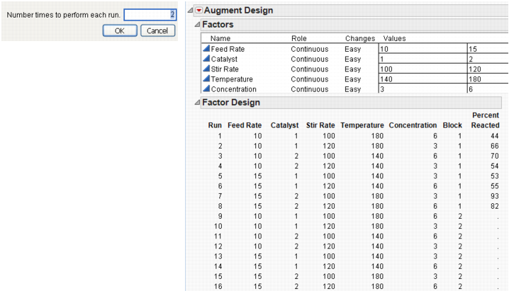
6. Enter the axial values in units of the factors scaled from –1 to +1, then enter the number of center points you want. When you click OK, the augmented design includes the number of center points specified and constructs two axial points for each variable in the original design.
Figure 15.22 Entering Axial Values

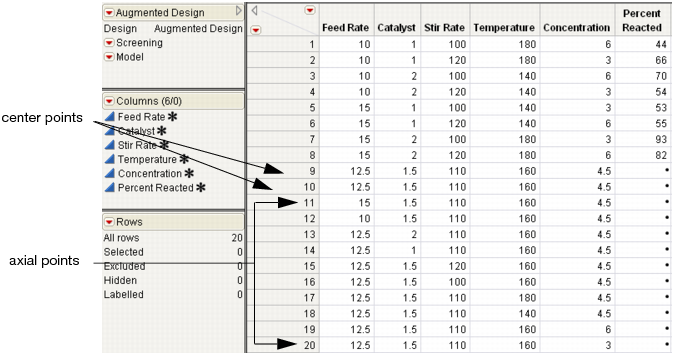
7. Click Make Table. The design table appears. Figure 15.23 shows a table augmented with two center points and two axial points for five variables.
Figure 15.23 Design Augmented With Two Center and Ten Axial Points
Adding New Runs and Terms
A powerful use of the augment designer is to add runs using a model that can have more terms than the original model. For example, you can achieve the objectives of response surface methodology by changing a linear model to a full quadratic model and adding the necessary number of runs. Suppose you start with a two-factor, two-level, four-run design. If you add quadratic terms to the model and five new points, JMP generates the 3 by 3 full factorial as the optimal augmented design.
D-optimal augmentation is a powerful tool for sequential design. Using this feature you can add terms to the original model and find optimal new test runs with respect to this expanded model. You can also group the two sets of experimental runs into separate blocks, which optimally blocks the second set with respect to the first.
To add new runs and terms to the original model:
1. Open a data table that contains a design you want to augment. This example uses Reactor Augment Data.jmp, from the Design Experiment Sample Data folder installed with JMP.
2. Select DOE > Augment Design.
3. In the initial Augment Design dialog, identify the response and factors you want to use for the augmented design (see Figure 15.15) and click OK.
4. If you want the original runs and the resulting augmented runs to be identified by a blocking factor, check the box beside Group New Runs into Separate Block (not used in this example).
5. Click the Augment button. The original number of runs (Figure 15.24) appear in the Factor Design panel.
Figure 15.24 Viewing the Existing Design

6. In the Design Generation panel, enter the number of total runs you want this design to contain. The number you enter is the original number of runs plus the number of additional runs you want.
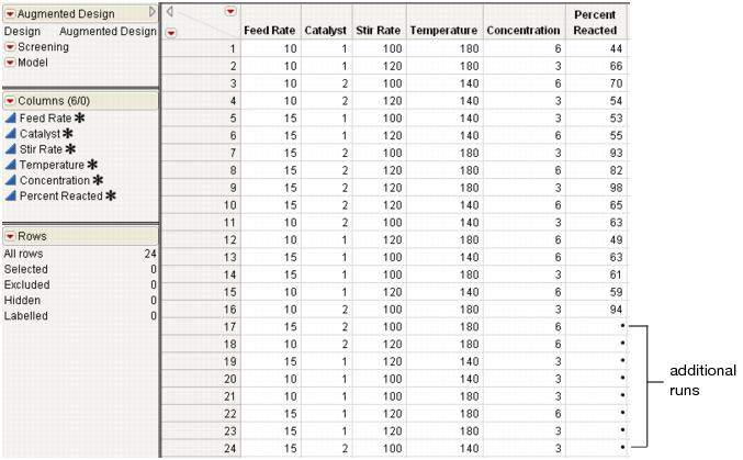
7. Click the Make Design button. The new number of runs (Figure 15.25) appear in the Design panel.
Figure 15.25 24 Total Runs
8. If desired, view the prediction variance profile and the prediction variance surface.
9. Click Make Table to create the augmented design JMP table (Figure 15.26) with the additional runs.
Figure 15.26 The Augmented Design Table with New Runs
Note: The Augment designer does not support designs that have terms whose estimability has been set to If Possible instead of Necessary, as is done in some screening designs that have fewer runs than terms.
Special Augment Design Commands
The Augment Design red triangle menu has several options, many of which are commands for saving and loading information about variables. They are available in all designs and more information is in Special Custom Design Commands. The following sections describe commands found in this menu that are specific to augment designs.
Save the Design (X) Matrix
To create a script and save it as a table property in the JMP design data table, click the red triangle icon in the Augment Design title bar and select Save X Matrix. Two or three scripts are saved to the table. Moments Matrix and Design Matrix scripts are always saved. If the design is a split plot design, an additional V Inverse script is also saved. When you run the Moments Matrix script, JMP creates a matrix called Moments and displays its number of rows in the log. When you run the Design Matrix script, JMP creates a matrix called X and displays its number of rows in the log. When you run the V Inverse script, JMP creates the inverse of the variance matrix of the responses, and displays its number of rows in the log. If you do not have the log visible, select View > Log or Window > Log on the Macintosh.
Modify the Design Criterion (D- or I- Optimality)
To modify the design optimality criterion, click the red triangle icon in the Augment Design title bar and select Optimality Criterion, then choose Make D-Optimal Design or Make I-Optimal Design. The default criterion for Recommended is D-optimal for all design types unless you have used the RSM button in the Model panel to add effects that make the model quadratic.
Select the Number of Random Starts
To override the default number of random starts, click the red triangle icon in the Augment Design title bar and select Number of Starts. A window appears with an edit box for you to enter the number of random starts for the design you want to build. The number you enter overrides the default number of starts, which varies depending on the design.
For additional information on the number of starts, see Why Change the Number of Starts?.
Specify the Sphere Radius Value
Augment designs can be constrained to a hypersphere. To edit the sphere radius for the design in units of the coded factors (–1, 1), click the red triangle icon in the Augment Design title bar and select Sphere Radius. Enter the appropriate value and click OK.
Or, use JSL and submit the following command before you build a custom design:
DOE Sphere Radius = 1.0;
In this statement you can replace 1.0 with any positive number.
Disallow Factor Combinations
In addition to linear inequality constraints on continuous factors and constraining a design to a hypersphere, you can define general factor constraints on the factors. You can disallow any combination of levels of categorical factors if you have not already defined linear inequality constraints.
For information on how to do this, see Disallowed Combinations: Accounting for Factor Level Restrictions.
..................Content has been hidden....................
You can't read the all page of ebook, please click here login for view all page.