
Surface tests to determine transport properties of concrete – II: analytical models to calculate permeability
Abstract:
This chapter presents theoretical models for the four tests described in Chapter 3. These are analytical models which use integrated forms of the equations presented in Chapter 1. Two additional tests are described to be used to assess the accuracy of the models; these are a sorptivity test and a high pressure permeability test. The models are used to calculate the sensitivity of the different tests to changes in concrete properties. For practical use the results indicate that the water tests give better results than the gas tests. No clear advantage of either drilled hole or surface tests was observed.
Key words
initial surface absorption test (ISAT); Figg test; analytical models; sorptivity test; high pressure permeability test
4.1 Introduction
The modelling of all four tests is based on the Darcy equation for pressure-driven flow (equation 1.1). For the vacuum decay tests the applied pressure is atmospheric and for the water absorption tests it is capillary suction.
4.2 Additional tests
For comparison with the surface tests two additional tests were used: sorptivity and a high pressure test.
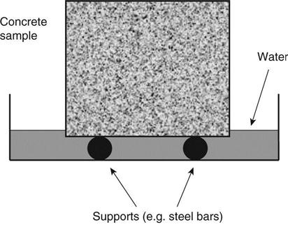
4.2.1 The sorptivity test
This test is shown in Fig. 4.1. The water rises into the concrete sample with capillary suction and the increase of mass is plotted against time. Measurements were carried out using specimens (50ϕ × 150 mm) which were oven dried and then rested on rods in water containers to allow free access of water to the inflow surface (see Fig. 4.1). The water level was maintained to remain at no more than about 5 mm above the base of the specimens. The lower areas on the sides of the specimens were coated with grease to achieve unidirectional flow. The cumulative water absorbed was recorded at different time intervals up to 2 h by weighing the specimens after removing the surface water using a dampened tissue.
The sorptivity is defined as the slope of the cumulative volume of water absorbed per unit area against the square root of time:
[4.1]
where S is the sorptivity (m s−0.5).
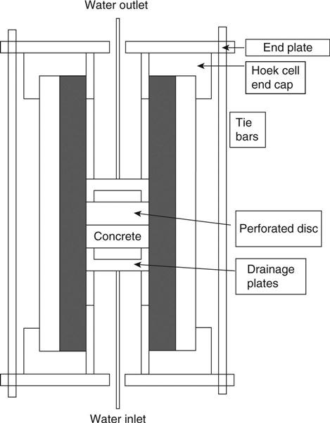
4.2.2 The high pressure permeability apparatus
The permeability of the samples was measured with water using 54 mm or 100 mm diameter cylindrical sections approximately 30 mm long in modified ‘Hoek’ triaxial cells (Figs 4.2–4.4).
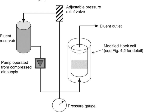

Pressures up to 10 MPa were used depending on the compressive strength of the particular specimen. These high pressures were chosen in order to give results in a practical timescale. Measurements of the effect of pressure on the results were made to relate them to the site application (see Chapter 9). The water pump was operated by a pressurised air supply.
To maintain the structural integrity of the sample, and prevent flow past its sides, a confining (triaxial) pressure was applied around an impermeable sleeve surrounding the sample. By maintaining the pore solution pressure below that of the confining pressure, the internal structure of the material was maintained. Note that with this apparatus, if the confining pressure is released rapidly during a high pressure test the pressure in the pores will cause concrete samples to break up.
The modifications to the Hoek cells were designed to provide a fluid supply to, and drain from, the samples and to contain the axial load to permit use without an external compression frame. On the downstream (top) face of the sample, this load could have caused spalling from the surface due to the high pressure in the pores so it was carried through a thick perforated disc. A porous (sinter) disc was placed against the sample to permit free flow across the face. From the perforated disc the load was carried by the drainage plates and then through load-bearing spacers to a substantial (20 mm thick) end plate with tie bars around the circumference.
The pressure was controlled by adjusting a pressure relief valve which recirculated fluid back to the reservoir (Fig. 4.3). This method was chosen because the pump maintained a more constant pressure when some flow was permitted, and also because it ensured safe operation. All of the components and pipework were made with stainless steel to permit the use of corrosive leachates in the experiments as an alternative to water.
Water was collected to approximately equate to one sample size, then the time required to collect 10 ml of water was recorded to calculate the intrinsic permeability from equation (1.4) as follows:
[4.2]
where:
K is the intrinsic permeability (m2)
VF is the velocity of Darcy flow (m/s), obtained as volume/(cross-sectional area × time)
x is the sample thickness (m)
P is the applied water pressure (Pa) and
e is the viscosity (Pa s).
4.3 Modelling of the absorption tests
There are numerous mechanisms which may contribute to the movement of water through concrete, including pressure-driven flow, capillary suction, osmosis, electro-osmosis and thermal migration. For simplicity, this model assumes that the flow is driven by capillary suction and controlled by permeability. The rate of capillary suction is initially high but decreases as the water filled volume of capillaries increases. Levitt (1970) derived equation (4.3) for the ISAT test (see Section 3.2) based on the mathematical formula from the Pouseille equation for a liquid travelling through a single capillary tube:
[4.3]
where:
ISA is the initial surface absorption (m3/m2/s)
t is the absorption time (s)
a, n are regression parameters
A is the area under cap (m2) and
FV is the flow rate (m3/s).
Thus, integrating:
[4.4]
4.3.1 The general model for water flow
The pressure head from capillary suction is given by equation (1.34). (The 200 mm head of water in the ISAT and CAT tests is assumed to be substantially less than P.)
In the model, it is assumed that, at any given time t after the start of the test, a volume V of the concrete is saturated with water and there is no water outside it. This assumption of a well-defined front to the water penetration is in agreement with the observations on samples which had been broken open during the test. Thus:
[4.5]
where ε is the porosity.
The flow through the concrete to the penetration front will be limited by the permeability (equation 1.4).
4.3.2 Modelling the ISAT and absorption
For the absorption test and the ISAT, the flow may be considered as one-dimensional (i.e. the curved wetting front is assumed to be flat, see experimental observations in Fig. 4.4). The area is thus constant and from equations (1.34) and (1.9):
[4.6]
where:
X is the distance in m from the reservoir to the wetting front and
A is the constant area.
Also:
[4.7]
Differentiating equation (4.6) with respect to t and combining it with equations (4.5) and (4.7) gives:
[4.8]
where:
[4.9]
The solution to this is:
[4.10]
Substituting into equation (4.3):
[4.11]
and n = 1/2.
Thus:
[4.12]
The absorption ISA10 is FV/A when t = 600 s.
4.3.3 Modelling the CAT test
For the CAT test (see Section 3.4.1) the area across which the water is flowing is approximately cylindrical (i.e. it is assumed that the observed section in Fig. 4.5 has parallel sides). If the wetting front is a distance x from the centre of the drilled hole and the depth of the hole is L the area will be:
[4.13]
Substituting into equation (1.9) and integrating with respect to x:
[4.14]
where:
x0 is the radius of the drilled hole.
Combining with equation (1.34) and differentiating with respect to time:
[4.15]
where:
[4.16]
The volume of concrete inside the wetting front will be:
[4.17]
where V0 is the volume of the drilled hole.
Combining with equations (4.5) and (4.15) this gives:
[4.18]
where:
[4.19]
The solution to this is:
[4.20]
For an approximate solution, the exponential may be expanded as the initial terms of a power series:
[4.21]
Substituting and rearranging gives:
[4.22]
During the initial part of a test when t is small δ/F will be ≈ 0 and the last term may be omitted. This solution may be seen to be the same as the one-dimensional solution in equation (4.10) with an area of 2πx0L (the area of the curved surface of the drilled hole).
4.4 Experimental testing for absorption
4.4.1 Preparation of test samples
To provide experimental confirmation of this analysis two concrete types, namely, Portland cement control (PC) and low water concrete (LWC), both of grade 35, were tested (Table 4.1). The test specimens (dimensions are detailed in each test procedure) were cast and kept under wet hessian for 1 day before demoulding. Two curing conditions were used: water curing at 20 °C (CC1) and air curing at 20 °C, 55 % RH (CC2), until testing at 28 days. The tests were carried out on duplicate specimens.

4.4.2 Test procedures
• Measurements of ISAT were carried out using samples (100 mm cubes) preconditioned in the oven at 105 °C until constant weight. To simulate a unidirectional flow, ISAT specimens were 100 mm cubes and the surface portion, not under the ISAT cap, was coated with grease. The initial surface absorption (ISA) was recorded at 10, 30, 60 and 120 min.
• CAT results were obtained in the same way as ISAT using 100 mm cubes conditioned in the oven exactly as for the ISAT samples.
• Measurements of water sorptivity were carried out as described in Section 4.2.1 on samples which had also been oven dried in the same way as the ISAT samples.
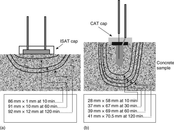
• A series of tests were carried out on concrete cubes in order to assess the shape of the wetting front after ISAT and CAT applications. This was done by splitting the test specimens at different intervals of time (e.g. 10, 30, 60 and 120 min) to observe the depth and width of water penetration.
• The permeability was measured at high pressure as described in Section 4.2.
4.4.3 Experimental results
The relationships between ISA, CAT and time followed equation (4.3) with a high correlation coefficient (r = 0.99). In order to compare the results from the different experiments, it was necessary to express the absorption results in differential form. If the flow rate is assumed to be of the same form as equation (4.3), this may be integrated to give the measured weight gain (equation 4.4).
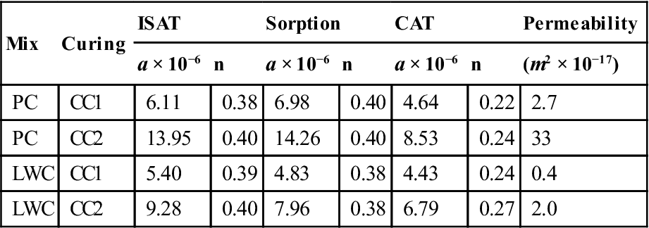
The absorption results showed a high correlation with this equation and results for a and n were obtained. The results for a and n from each of the three tests are given in Table 4.2. It may be seen that there is excellent agreement between the absorption results and the ISAT results and higher flow rates for the CAT.
Table 4.2
| Mix | Curing | ISAT | Sorption | CAT | Permeability | |||
| a × 10−6 | n | a × 10−6 | n | a × 10−6 | n | (m2 × 10−17) | ||
| PC | CC1 | 6.11 | 0.38 | 6.98 | 0.40 | 4.64 | 0.22 | 2.7 |
| PC | CC2 | 13.95 | 0.40 | 14.26 | 0.40 | 8.53 | 0.24 | 33 |
| LWC | CC1 | 5.40 | 0.39 | 4.83 | 0.38 | 4.43 | 0.24 | 0.4 |
| LWC | CC2 | 9.28 | 0.40 | 7.96 | 0.38 | 6.79 | 0.27 | 2.0 |
The type and curing of concrete has a significant influence on the depth of water penetration. Typical wetting front shapes for ISAT and CAT applications for water-cured concrete of grade 35 are shown in Fig. 4.5. It may be seen that the wetting front shape is parabolic with a wide base on the concrete surface. This is attributed to the fact that the skin layer is more porous (due to bleeding channels, entrapped air, aggregate settlement, etc.). The wetting front for the ISAT is assumed to be flat in the analysis and for the CAT it is assumed to be cylindrical, but these are shown by the results to be quite good approximations.
4.4.4 Results for the model
The solutions given in equations (4.12) and (4.20) have been compared with the experimental results in Table 4.2 plotted from equation (4.3). The results are in Figs 4.6–4.9 which show flow per unit area plotted against time. For the CAT results, this area is the area of the curved surface of the drilled hole. These figures were obtained with the following fixed parameters:
• At 20 °C the viscosity of water e = 10−3 Pa s and
• the surface tension of water s = 0.073 N/m.
• The area under the ISAT cap A = 5.8 × 10⁻³m.
• The depth of the drilled hole for CAT, L = 0.05 m and the radius, x0 was 6.5 × 10⁻³m.


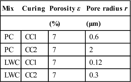
The other variables are the pore radius and the porosity. The values used for these are given in Table 4.3. The flow rate depends on the ratio of the two and neither was measured so a constant porosity of 7 % has been assumed which is typical for concrete. The different values for pore radius were set to give agreement with the model for the ISAT test. The pore radii obtained in this way are at the upper end of the range of pore sizes found in concrete. This is consistent with the assumptions of the model because, if the radius of a pore varies along its length, the capillary suction pressure to draw water along it will correspond to the largest radius. It may be seen that the model gives a lower pore radius for the LWC and for the better curing condition (CC1).
Table 4.3
| Mix | Curing | Porosity ε | Pore radius r |
| (%) | (μm) | ||
| PC | CC1 | 7 | 0.6 |
| PC | CC2 | 7 | 2 |
| LWC | CC1 | 7 | 0.12 |
| LWC | CC2 | 7 | 0.3 |
It may be seen that the model gives a far more accurate prediction of the difference between ISAT and CAT for the water-cured samples. The reason for this is not known, but it is unlikely that different fundamental processes are responsible because all of the samples were dried before testing.
4.5 Tests using a vacuum to measure air flow
4.5.1 Approximations
The main approximations used for modelling the tests are an assumption of steady state for the gas flow and simplifications of the geometry. The steady state assumption is that, at any time, the mass of gas flowing into the section of the sample which is being tested is equal to the amount of gas flowing out of it. This is justified on the basis that the rate of change of pressure is relatively slow (the duration of the test is measured in minutes) and the volume through which the gas is flowing is relatively small. This assumption has been used extensively in the literature (e.g. Bamforth, 1987). The geometrical assumptions are that the flow to the surface tests is one-dimensional (towards the surface) and the flow to the drilled hole tests is radial towards the hole. These assumptions have been made in the context of the use to which the models have been put (evaluating sensitivity to concrete properties).
4.5.2 General model for the vacuum tests
In these tests, the permeating fluid is compressible and the observed flux FV in m3/s will therefore change with pressure. The flow is therefore best expressed as molecular flow where J is the total flux in mol/m2/s and dn/dt is the flow rate of the gas (mol/s). Both J and dn/dt are approximately constant across the sample (assuming a steady state within it). Thus the flow dn/dt is given by equation (1.11).
The change of pressure in the vacuum chamber will be given by
[4.23]
where:
V is the evacuated volume and
P is the pressure in it.
In order to apply these equations, it is now assumed that the gas is flowing into the vacuum from a region a distance X metres away where there is a large reservoir of gas at atmospheric pressure. Tests to measure X are presented in Chapter 5.
4.5.3 The APNS test
In this test (see Section 3.4.2), the flow is approximately one-dimensional out of the concrete towards the vacuum. The area A is therefore approximately constant. Integrating equation (1.9) across the sample gives:
[4.24]
Combining this with equation (4.23) gives:
[4.25]
The integral of this expression gives:
[4.26]
where:
Pi is the initial vacuum and
Patm is atmospheric pressure.
The APNS index is the value of t when P reaches 90 kPa from an initial Pi = 1 kPa.
4.5.4 Modelling the Figg test
The Figg test (see Section 3.3) has an approximately cylindrical geometry. Thus:
[4.27]
and
[4.28]
where:
x is the radius at which the flow is being considered
L is the length of the evacuated volume in m and
x0 is its radius.
Following through the integration as for the APNS test gives:
[4.29]
A further analysis of this is given in Chapter 5 in which the accuracy is improved by including a second integral of a spherical region at the base of the hole. The Figg permeation index is the value of t when P reaches 55 kPa from an initial Pi = 45 kPa.
4.6 The choice of test for practical applications
When deciding which surface test to use on a given structure (selecting from the four in Table 3.1), the most important consideration may be the existence of local knowledge or standards; this is not considered here. The damage to the structure caused by the tests is on a similar scale for all four tests since the two which do not involve drilling a hole result in an unsightly grease deposit on the surface which is difficult to remove. The amount of work involved in carrying out each of the tests is also similar. The following discussion therefore only considers the ability of the tests to determine the potential durability.
While all of the tests measure permeability, it may be seen that two measure this for gas and two for water. Bamforth (1987) has published a very comprehensive discussion of the effect of gas slippage and gives a graph to correct for it at different pressures. In Table 4.4 two different concretes, A and B, are considered with water permeabilities of 10−17 and 10−18m2. These permeabilities are typical for grade 35 and 60 concretes (Bamforth, 1987). The corresponding gas permeabilities, the calculated results for the four tests for each concrete using the equations derived in this chapter and the average measured coefficient of variation for the tests on the concretes reported in Chapter 3 (using vacuum drying) are also given in the table. The variation for the ISAT was obtained from the tests described in Section 3.5.
Table 4.4
| Material | Water permeability K (m2) | ISAT10 min reading ISA10 10−2 ml/m2/s | CAT10 min reading CAT10 10−2 ml/m2/s | Gas permeability at 0.5 atmospheres absolute K (m2) | APNS permeation index (s) | Figg permeation index (s) |
| Concrete A | 10−17 | 37 | 59 | 2 × 10⁻¹⁶ | 7300 | 120 |
| Concrete B | 10−18 | 12 | 14 | 10−16 | 14 600 | 240 |
| Ratio A/B | 3.1 | 4.2 | 0.5 | 0.5 | ||
| Average V % (vacuum-dried) | 15.7 | 14.1 | – | 19.1 |

The values used for the calculations in Table 4.4 were:
| R | gas constant | 8.31 J/mol/K |
| T | temperature | 293 K |
| e | viscosity of water | 10−3 Pa s |
| s | surface tension of water | 0.073 N/m |
| A | area under ISAT test cap | 5.8 × 10⁻³ m2 |
| V | volume under ISAT test cap | 2.9 × 10⁻⁵ m3 |
| L | depth of drilled hole | 50 mm |
| x0 | radius of drilled hole | 6.5 mm |
| Patm | atmospheric pressure | 100 kPa |
| Pi | initial vacuum | 45 kPa for Figg test and 1 kPa for APNS test |
| P | final pressure | 55 kPa for Figg test and 90 kPa for APNS test |
| α | porosity | 7 % |
| r | radius of largest pores | 0.6 μm (see Table 4.3) |
The unknown constant is X, the distance over which the pressure drop occurs in the gas tests. If no value of X is used, K/X may be used as a measure of permeability rather than K. This approach cannot be used for the Figg test because the cylindrical geometry gives a logarithmic relationship in equation (4.26). For the present discussion, the value is not important and a realistic estimate of 10 mm has been used. An extensive investigation which used computer modelling to avoid the necessity to use a simplified ‘permeation block’ of finite thickness is presented in Chapter 6, and it is concluded that for low porosity concretes, such as those used in the work reported here, the effect of the approximation is not substantial. In Chapter 5 a new method is presented to measure the value of X directly.
Table 4.4 shows that the derived equations give realistic values for the different test results. The conclusion from the table is that the water tests, in particular the CAT test, should give better distinction between different concrete qualities because of the higher proportional change in the measured value for a given change in concrete permeability. The coefficient of variation may also be seen to be lower for the water tests (data is not currently available for the APNS test). It must be observed, however, that the tests measure different properties in that the water tests measure capillary suction as well as permeability. If possible, a site test programme should therefore use both tests. These results do not indicate a very clear preference for either surface or drilled hole tests. It may be argued that the drilled hole tests will be less affected by surface effects or contamination, but the surface tests measure the ingress of fluids into a structure more realistically.
4.7 Conclusions
• Analytical solutions have been presented for the main surface permeability tests and these gave realistic values for permeability.
• It was found that a full solution to the vacuum tests was not possible because the distance over which the vacuum decays is not known. This problem is addressed in Chapter 5.
• An analysis of the different tests concluded that the water tests would give more consistent results.