
Electrical tests to analyse the transport properties of concrete – II: using a neural network model to derive diffusion coefficients
Abstract:
In this chapter, the computer model of electromigration which was introduced in Chapter 10 is combined with an artificial neural network (ANN) model to enable values for diffusion coefficients to be determined from test results from the modified ASTM C1202 rapid chloride test. The ANN is necessary because the model in Chapter 10 requires values for the diffusion coefficients and capacity factors of the mobile ions and uses these to predict the test results for current and membrane potential. By using the ANN, it is possible to use the test results to calculate the diffusion coefficients and capacity factors from the test results.
Key words
artificial neural networks; optimisation; membrane potential; capacity factor; diffusion; electromigration
11.1 Introduction
The methods presented in Chapter 10 can be used to predict the current–time transient and the mid-point voltage during a rapid chloride test. The calculations require input values of the diffusion coefficients and capacity factors of all the ions. However, the usual requirement in practical applications would be to obtain the coefficients from experimental results. Thus a prediction method was used. There are many possibilities for this. Section 6.3.2 describes how the output from a numerical model was optimised by repeatedly running it until the results were seen to be close to those observed. Section 15.3 refers to an optimisation routine that worked by progressively optimising each variable. This could only work for a small number of variables and was very slow. There are many other possibilities, including the response surface method. However, the fastest and most efficient method is to use an artificial neural network (ANN).
11.2 Experimental method
11.2.1 Concrete mixes
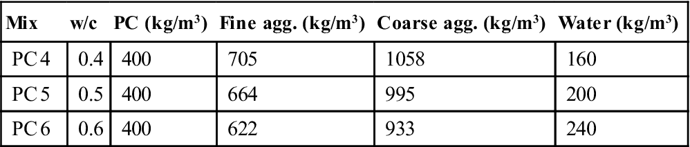
Samples of Portland cement (PC) with different water to cement (w/c) ratios were mixed. Table 11.1 shows the mix designs and the nomenclature used in this study. All the tests were made on samples around 6 months old which were kept in a controlled humidity and temperature room until each test was started. During the mixing, depending on the water content, the mixes had different flow properties. In order to avoid affecting the strength because of the differences in the mix compaction, all the mixes were compacted mechanically with a vibrating table. The moulds were filled with concrete in three layers and compacted to remove the air and reach the maximum density.
11.2.2 Current and membrane potential in the ASTM C1202 test
The ASTM C1202 test is described in Section 10.2. Each test was run twice and the result shown is the average of both results.
11.2.3 Porosity measurement
The porosity was measured by weight loss as in Section 7.3.3.
11.3 Neural network optimisation model
The computational model used two main techniques. The electro-diffusion numerical routine described in Section 10.5 was used. However, because in reality the physical transport properties are unknown, a neural network algorithm was trained to optimise those physical properties. As a result of combining both techniques, the transport properties of a concrete sample could be determined from experimental observations of mid-point membrane potential and current measured simultaneously during a migration test.
To train the network, the numerical electro-diffusional model was run many times in order to obtain a database of the input and the corresponding target vectors. During the training, the outputs of the model were used as inputs for the neural network. All the data was normalised between −1 and +1 in order to avoid the influence of the scale of the physical quantities. In the same way, the tangential transfer function was limited to be between −1 and +1. The Levenberg-Marquardt training algorithm was used. Figure 11.1 shows a conceptual diagram of the integrated model.

The optimisation model used a feed-forward back-propagation network with a multilayer architecture. Six neurons defined the input layer, corresponding to values of the current and the mid-point membrane potential at different times. A middle hidden layer had three neurons, and the output layer has seven neurons corresponding to the intrinsic diffusion coefficients of Cl−, OH−, Na+ and K+, the porosity, the hydroxide composition in the pore solution at the start of the test, and the binding capacity factor for chloride ions. The neural network model was constructed using the neural network tool box of Matlab®. Figure 11.2 shows the input, the hidden layer and the outputs of the network.

11.3.1 Integrated numerical and neural network model
Obtaining the related transport chloride properties of concrete from measurements of current has been reported (Yang et al., 2007); however, long durations and steady state conditions are required. In the present research, with the simultaneous measurement of the current and the mid-point membrane potential, it is possible to determine a unique combination of the transport properties by using a trained neural network. In order to simulate the transport properties of concrete and taking into account the complex variables related with the physical phenomenon, two assumptions were made:
1. The only ions that interact with the cement matrix products are chlorides, and that interaction is defined with a linear binding isotherm. Although it has been demonstrated experimentally (Delagrave et al., 1997) that non-linear isotherms reflect the absorption phenomena better, the model uses an average linear isotherm that represents in a good way the average adsorption of chlorides as described in Section 1.3.1.
2. At the start of the test, the chemical pore solution is composed of ions OH−, K+, and Na+ and, in order to keep electroneutrality, it was assumed that the concentration of hydroxyl ions is equilibrated with a proportion of 33 % of sodium and 66 % of potassium. This assumption was based on published results (Bertolini et al., 2013).
11.4 Results and discussion
11.4.1 Experimental determination of the transient current, membrane potential and the diffusion coefficients
The average current measured for each mix in the migration test is shown in Fig. 11.3. As was expected, an increase in the w/c ratio gave an increase in the current passed, and a corresponding increase in the temperature of the sample. The measured maximum value of temperature in the anode solution was 63, 44, and 36 °C for samples of w/c ratio of 0.6, 0.5 and 0.4, respectively, and the values of charge calculated as the area under the graph of current versus time were 9580, 6863 and 4149 C for samples of w/c ratio of 0.6, 0.5 and 0.4, respectively.

The measured membrane potential is shown in Fig. 11.4a. There was noise in the results as noted in Chapter 10. They were filtered with commercial curve fitting software in order to find the best trend, and this can be seen in Fig. 11.4b. The average membrane potential for each mix is shown in Fig. 11.4c, it can be seen that for all mixes the membrane potential showed a rise from its initial value; however, mix PC-6 showed an initial decrease during the first 2 h.

11.4.2 Prediction of chloride related properties
The trained neural network was fed with the values for the current transient and the mid-point voltage from the migration test and, from this data, the chloride transport related properties were calculated. As a measure of the reliability of the network, the transport properties obtained were used to run the electro-diffusional model in order to obtain a simulated transient current and mid-point membrane potential. The comparison of these curves is shown in Fig. 11.5. It can be seen that, for the current, the simulations are in very good agreement with the experiments and, for the membrane potential, although there are some small differences, there is a well-defined trend.

The differences between the measured and simulated membrane potential can be explained by factors related to the accuracy of the measurement device used during the experiment, the heating of the material under an electrical field, or the variability of the test. However, it may be seen that the neural network is able to give a good fit to the profile of the membrane potential, given that the number of possible combinations of properties that yield a given current and membrane potential is almost infinite.
The transport properties calculated by modelling the test results include the porosity, the binding capacity factor and the initial hydroxide composition at the start of the test. As was expected, the porosity increases with an increase of the water to binder (w/b) ratio (Fig. 11.6a). It can be seen that the trend of the measured porosity is similar to that calculated; however, some differences arise from errors in either the numerical or experimental methods. The binding capacity factor decreases as the w/b ratio increases, presumably due to the refining of the hydration compounds enabling them to bind more free chloride ions (Fig. 11.6b). The calculated initial chemical content of the pore solution increases with an increase in the w/b ratio. This can be attributed to the increased amount of water, which can keep more alkalis in the pore solution.

The calculated intrinsic diffusion coefficients for all the species involved in the simulation (Cl−, OH−, Na+, K+) are shown in Fig. 11.7. As observed by other researchers (Andrade, 1993), the anions generally had lower diffusion coefficients than chlorides and hydroxides. The exception to this was mix 6, where hydroxide and sodium have a similar diffusivity. As was expected, the calculated numerical values of the intrinsic coefficients for all the species are, for all the cases, lower than the coefficients of diffusion in infinite diluted solutions in electrochemistry textbooks (Bockris and Reddy, 1998). The values obtained are physically possible and are in acceptable ranges.

11.5 Conclusions
The experimental–numerical procedure gave viable results for the fundamental properties of concrete. The initial hydroxide composition of the pore solution, the chloride binding capacity, the porosity and the diffusion coefficients for all the species involved were calculated and gave results which were comparable with those reported elsewhere.