
In this chapter, we will explore Support Vector Machines (SVMs). We will study several SVM implementations in Clojure that can be used to build and train an SVM using some given training data.
SVMs are supervised learning models that are used for both regression and classification. In this chapter, however, we will focus on the problem of classification within the context of SVMs. SVMs find applications in text mining, chemical classification, and image and handwriting recognition. Of course, we should not overlook the fact that the overall performance of a machine learning model mostly depends on the amount and nature of the training data and is also affected by which machine learning model we use to model the available data.
In the simplest form, an SVM separates and predicts two classes of data by estimating the optimal vector plane or hyperplane between these two classes represented in vector space. A hyperplane can be simply defined as a plane that has one less dimension than the ambient space. For a three-dimensional space, we would obtain a two-dimensional hyperplane.
A basic SVM is a non-probabilistic binary classifier that uses linear classification. In addition to linear classification, SVMs can also be used to perform nonlinear classification over several classes. An interesting aspect of SVMs is that the estimated vector plane will have a substantially large and distinct gap between the classes of input values. Due to this, SVMs often have a good generalization performance and also implement a kind of automatic complexity control to avoid overfitting. Hence, SVMs are also called large margin classifiers. In this chapter, we will also study how SVMs achieve this large margin between classes of input data, when compared to other classifiers. Another interesting fact about SVMs is that they scale very well with the number of features being modeled and thus, SVMs are often used in machine learning problems that deal with a large number of features.
As we previously mentioned, SVMs classify input data across large margins. Let's examine how this is achieved. We use our definition of a logistic classification model, which we previously described in Chapter 3, Categorizing Data, as a basis for reasoning about SVMs.
We can use the logistic or sigmoid function to separate two classes of input values, as we described in Chapter 3, Categorizing Data. This function can be formally defined as a function of an input variable X as follows:
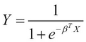
In the preceding equation, the output variable ![]() depends not only on the variable
depends not only on the variable ![]() , but also on the coefficient
, but also on the coefficient ![]() . The variable
. The variable ![]() is analogous to the vector of input values in our model, and the term
is analogous to the vector of input values in our model, and the term ![]() is the parameter vector of the model. For binary classification, the value of Y must exist in the range of 0 and 1. Also, the class of a set of input values is determined by whether the output variable
is the parameter vector of the model. For binary classification, the value of Y must exist in the range of 0 and 1. Also, the class of a set of input values is determined by whether the output variable ![]() is closer to 0 or 1. For these values of Y, the term
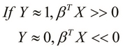
is closer to 0 or 1. For these values of Y, the term ![]() is either much greater than or much less than 0. This can be formally expressed as follows:
is either much greater than or much less than 0. This can be formally expressed as follows:
For ![]() sample with input values
sample with input values ![]() and output values
and output values ![]() , we define the cost function
, we define the cost function ![]() as follows:
as follows:
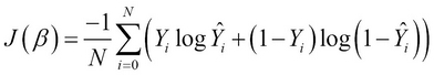
For a logistic classification model, ![]() is the value of logistic function when applied to a set of input values
is the value of logistic function when applied to a set of input values ![]() . We can simplify and expand the summation term
. We can simplify and expand the summation term ![]() in the cost function defined in the preceding equation, as follows:
in the cost function defined in the preceding equation, as follows:
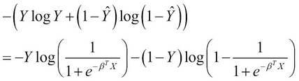
It's obvious that the cost function shown in the preceding expression depends on the two logarithmic terms in the expression. Thus, we can represent the cost function as a function of these two logarithmic terms, represented by the terms ![]() and
and ![]() . Now, let's assume the two terms as shown the following equation:
. Now, let's assume the two terms as shown the following equation:
Both the functions ![]() and
and ![]() are composed using the logistic function. A classifier that models the logistic function must be trained such that these two functions are minimized over all possible values of the parameter vector
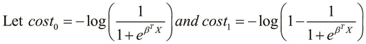
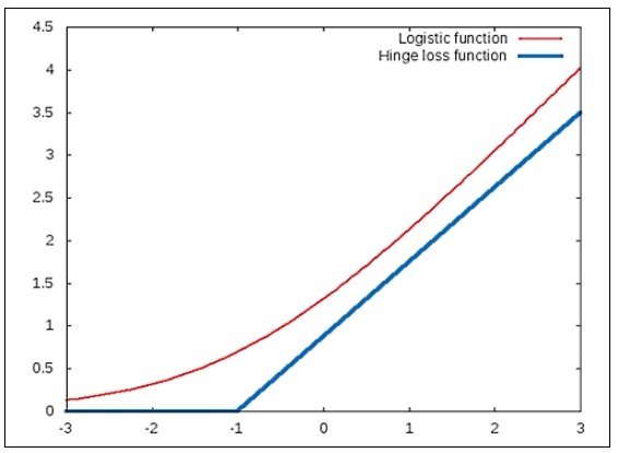
are composed using the logistic function. A classifier that models the logistic function must be trained such that these two functions are minimized over all possible values of the parameter vector ![]() . We can use the hinge-loss function to approximate the desired behavior of a linear classifier that uses the logistic function (for more information, refer to "Are Loss Functions All the Same?"). We will now study the hinge-loss function by comparing it to the logistic function. The following diagram depicts how the
. We can use the hinge-loss function to approximate the desired behavior of a linear classifier that uses the logistic function (for more information, refer to "Are Loss Functions All the Same?"). We will now study the hinge-loss function by comparing it to the logistic function. The following diagram depicts how the ![]() function must vary with respect to the term
function must vary with respect to the term ![]() and how it can be modeled using the logistic and hinge-loss functions:
and how it can be modeled using the logistic and hinge-loss functions:
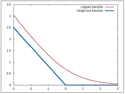
In the plot shown in the preceding diagram, the logistic function is represented as a smooth curve. The function is seen to decrease rapidly before a given point and then decreases at a lower rate. In this example, the point at which this change of rate of the logistic function occurs is found to be x = 0. The hinge-loss function approximates this by using two line segments that meet at the point x = 0. Interestingly, both these functions model a behavior that changes at a rate that is inversely proportional to the input value x. Similarly, we can approximate the effect of the ![]() function using the hinge-loss function as follows:
function using the hinge-loss function as follows:
Note that the ![]() function is directly proportional to the term
function is directly proportional to the term ![]() . Thus, we can achieve the classification ability of the logistic function by modelling the hinge-loss function and a classifier built using the hinge-loss function will perform equally well as a classifier using the logistic function.
. Thus, we can achieve the classification ability of the logistic function by modelling the hinge-loss function and a classifier built using the hinge-loss function will perform equally well as a classifier using the logistic function.
As seen in the preceding diagram, the hinge-loss function only changes its value at the point ![]() . This applies to both the functions
. This applies to both the functions ![]() and
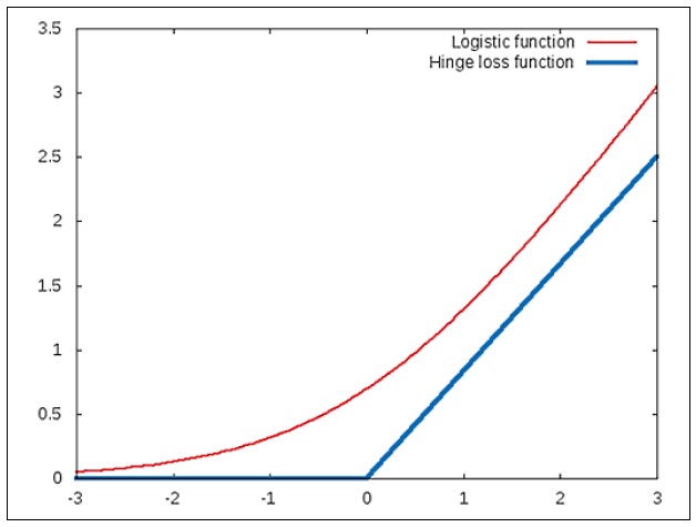
and ![]() . Thus, we can use the hinge loss function to separate two classes of data depending on whether the value of
. Thus, we can use the hinge loss function to separate two classes of data depending on whether the value of ![]() is greater or less than 0. In this case, there's virtually no margin of separation between these two classes. To improve the margin of classification, we can modify the hinge-loss function such that its value is greater than 0 only when
is greater or less than 0. In this case, there's virtually no margin of separation between these two classes. To improve the margin of classification, we can modify the hinge-loss function such that its value is greater than 0 only when ![]() or
or ![]() .
.
The modified hinge-loss functions can be plotted for the two classes of data as follows. The following plot describes the case where ![]() :
:
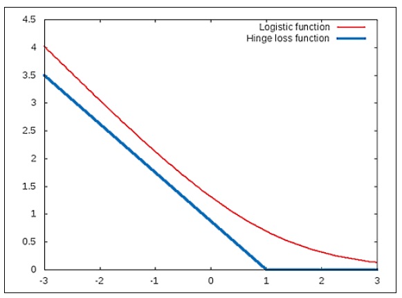
Similarly, the modified hinge-loss function for the case ![]() can be illustrated by the following plot:
can be illustrated by the following plot:
Note that the hinge occurs at -1 in the case of ![]() .
.
If we substitute the hinge-loss functions in place of the ![]() and
and ![]() functions, we arrive at an optimization problem of SVMs (for more information, refer to "Support-vector networks"), which can be formally written as follows:
functions, we arrive at an optimization problem of SVMs (for more information, refer to "Support-vector networks"), which can be formally written as follows:
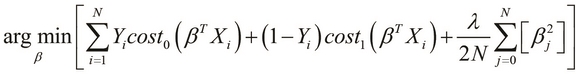
In the preceding equation, the term ![]() is the regularization parameter. Also, when
is the regularization parameter. Also, when ![]() , the behavior of the SVM is affected more by the
, the behavior of the SVM is affected more by the ![]() function than the
function than the ![]() function, and vice versa when
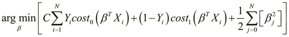
function, and vice versa when ![]() . In some contexts, the regularization parameter
. In some contexts, the regularization parameter ![]() of the model is added to the optimization problem as a constant C, where C is analogous to
of the model is added to the optimization problem as a constant C, where C is analogous to ![]() . This representation of the optimization problem can be formally expressed as follows:
. This representation of the optimization problem can be formally expressed as follows:
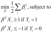
As we only deal with two classes of data in which ![]() is either 0 or 1, we can rewrite the optimization problem described previously, as follows:
is either 0 or 1, we can rewrite the optimization problem described previously, as follows:
Let's try to visualize the behavior of an SVM on some training data. Suppose we have two input variables ![]() and
and ![]() in our training data. The input values and their classes can represented by the following plot diagram:
in our training data. The input values and their classes can represented by the following plot diagram:
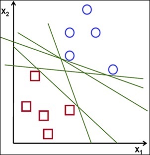
In the preceding plot diagram, the two classes in the training data are represented as circles and squares. A linear classifier will attempt to partition these sample values into two distinct classes and will produce a decision boundary that can be represented by any one of the lines in the preceding plot diagram. Of course, the classifier should strive to minimize the overall error of the formulated model, while also finding a model that generalizes the data well. An SVM will also attempt to partition the sample data into two classes just as any other classification model. However, the SVM manages to determine a hyperplane of separation that is observed to have the largest possible margin between the two classes of input data.
This behavior of an SVM can be illustrated using the following plot:
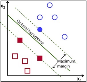
As shown in the preceding plot diagram, an SVM will determine the optimal hyperplane that separates the two classes of data with the maximum possible margin between these two classes. From the optimization problem of an SVM, which we previously described, we can prove that the equation of the hyperplane of separation estimated by the SVM is as follows:
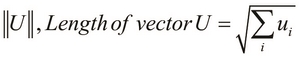
To understand more about how an SVM achieves this large margin of separation, we need to use some elementary vector arithmetic. Firstly, we can define the length of a given vector as follows:
Another operation that is often used to describe SVMs is the inner product of the two vectors. The inner product of two given vectors can be formally defined as follows:
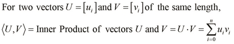
As shown in the preceding equation, the inner product ![]() of the two vectors
of the two vectors ![]() and
and ![]() is equal to the dot product of the transpose of
is equal to the dot product of the transpose of ![]() and the vector
and the vector ![]() . Another way to represent the inner product of two vectors is in terms of the projection of one vector onto another, which is given as follows:
. Another way to represent the inner product of two vectors is in terms of the projection of one vector onto another, which is given as follows:
Note that the term ![]() is equivalent to the vector product
is equivalent to the vector product ![]() of the vector V and the transpose of the vector U. Since the expression
of the vector V and the transpose of the vector U. Since the expression ![]() is equivalent to the product
is equivalent to the product ![]() of the vectors, we can rewrite the optimization problem, which we described earlier in terms of the projection of the input variables onto the output variable. This can be formally expressed as follows:
of the vectors, we can rewrite the optimization problem, which we described earlier in terms of the projection of the input variables onto the output variable. This can be formally expressed as follows:
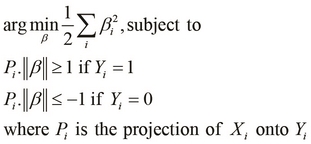
Hence, an SVM attempts to minimize the squared sum of the elements in the parameter vector ![]() while ensuring that the optimal hyperplane that separates the two classes of data is present in between the two planes and
while ensuring that the optimal hyperplane that separates the two classes of data is present in between the two planes and ![]() and
and ![]() . These two planes are called the support vectors of the SVM. Since we must minimize the values of the elements in the parameter vector
. These two planes are called the support vectors of the SVM. Since we must minimize the values of the elements in the parameter vector ![]() , the projection
, the projection ![]() must be large enough to ensure that
must be large enough to ensure that ![]() and
and ![]() :
:
Thus, the SVM will ensure that the projection of the input variable ![]() onto the output variable
onto the output variable ![]() is as large as possible. This implies that the SVM will find the largest possible margin between the two classes of input values in the training data.
is as large as possible. This implies that the SVM will find the largest possible margin between the two classes of input values in the training data.
We will now describe a couple of alternative forms to represent an SVM. The remainder of this section can be safely skipped, but the reader is advised to know these forms as they also widely used notations of SVMs.
If ![]() is the normal to hyperplane estimated by an SVM, we can represent this hyperplane of separation using the following equation:
is the normal to hyperplane estimated by an SVM, we can represent this hyperplane of separation using the following equation:
The two peripheral support vectors of this hyperplane have the following equations:
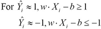
We can use the expression ![]() to determine the class of a given set of input values. If the value of this expression is less than or equal to -1, then we can say that the input values belong to one of the two classes of data. Similarly, if the value of the expression
to determine the class of a given set of input values. If the value of this expression is less than or equal to -1, then we can say that the input values belong to one of the two classes of data. Similarly, if the value of the expression ![]() is greater than or equal to 1, the input values are predicted to belong to the second class. This can be formally expressed as follows:
is greater than or equal to 1, the input values are predicted to belong to the second class. This can be formally expressed as follows:
The two inequalities described in the preceding equation can be combined into a single inequality, as follows:
Thus, we can concisely rewrite the optimization problem of SVMs as follows:
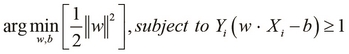
In the constrained problem defined in the preceding equation, we use the normal ![]() instead of the parameter vector
instead of the parameter vector ![]() to parameterize the optimization problem. By using Lagrange multipliers
to parameterize the optimization problem. By using Lagrange multipliers ![]() , we can express the optimization problem as follows:
, we can express the optimization problem as follows:
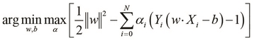
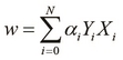
This form of the optimization problem of an SVM is known as the primal form. Note that in practice, only a few of the Lagrange multipliers will have a value greater than 0. Also, this solution can be expressed as a linear combination of the input vectors ![]() and the output variable
and the output variable ![]() , as follows:
, as follows:
We can also express the optimization problem of an SVM in the dual form, which is a constrained representation that can be described as follows:
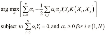
In the constrained problem described in the preceding equation, the function ![]() is called the kernel function and we will discuss more about the role of this function in SVMs in the later sections of this chapter.
is called the kernel function and we will discuss more about the role of this function in SVMs in the later sections of this chapter.