
The propagation-based approximation algorithm is a more generalized version of the belief propagation algorithm and works on the same principle of passing messages. In the case of exact inference, we used to construct a clique tree and then passed messages between the clusters. However, in the case of the propagation-based approximation algorithms, we will be performing message passing on cluster graphs.
Let's take the simple example of a network:

Fig 4.1: A simple Markov network
It is possible to construct multiple cluster graphs for this network. Let's take the example of the following two cluster graphs:

Fig 4.2: Cluster graphs for the network in Fig 4.1
Fig 4.2 shows two possible cluster graphs for the network in Fig 4.1. The cluster graph in Fig 4.2(a) is a clique tree and the clusters are (A, B, C) and (B, C, D). Whereas, the cluster graph in Fig 4.2(b) has four clusters (A, B), (B, C), (C, D), and (A, D). It also has loops:

Fig 4.3: Change of estimated probability with a number of iterations
Let's assume that the factors for the network are such that it's more likely for the variables to agree with the same state than different states, that is, ![]() and
and ![]() are much larger than
are much larger than ![]() and
and ![]() , and so on. Applying the message passing algorithm, messages will be passed from (A, B) to (B, C) to (C, D) to (A, D) and then again from (A, D) to (A, B). Also, let's consider that the strength of the message
, and so on. Applying the message passing algorithm, messages will be passed from (A, B) to (B, C) to (C, D) to (A, D) and then again from (A, D) to (A, B). Also, let's consider that the strength of the message ![]() increases the belief that b = 0. So now, when the cluster passes the message, it will increase the belief that c = 0 and so on. So finally, when the message reaches (A, B), it will increase the belief of A being 0, which in turn also increases the chances of B being 0. Hence, in each iteration, because of the loop in the network, the probability of A being 0 keeps on increasing until it reaches a convergence point, as shown in the graph in Fig 4.3.
increases the belief that b = 0. So now, when the cluster passes the message, it will increase the belief that c = 0 and so on. So finally, when the message reaches (A, B), it will increase the belief of A being 0, which in turn also increases the chances of B being 0. Hence, in each iteration, because of the loop in the network, the probability of A being 0 keeps on increasing until it reaches a convergence point, as shown in the graph in Fig 4.3.
In the case of exact inference, we had imposed two conditions on cluster graphs that led us to the clique trees. The first one was that the cluster graph must be a tree and should have no loops. The second condition was that it must satisfy the running intersection property. Now, in the case of the cluster graph belief propagation, we remove the first condition and redefine a more generalized running intersection property.
We say that a cluster graph satisfies a running intersection property if, whenever there is a variable X, and ![]() and
and ![]() , there is only one path from
, there is only one path from ![]() to
to ![]() through which messages about X flow.
through which messages about X flow.
This new generalized running intersection property leaves us another question, "how do we define sepsets now?". Let's take the example of the following two cluster graphs in Fig 4.4:
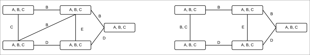
Fig 4.4: Two different clusters for the same network
In the case of exact inference, our sepsets used to be the common elements in the clusters. However, as we can see in the examples in the Fig 4.4, the same variable is common in multiple clusters. Therefore, to satisfy our running intersection property, we can't have it in the sepset of all the clusters.
In the case of clique trees, we performed inference by calibrating beliefs. Similarly, in the case of cluster graphs, we also say that the graph is calibrated if, for each edge (i, j) between the clusters ![]() and
and ![]() , we have the following:
, we have the following:

Looking at the preceding equation, we can also say that a cluster graph is calibrated if the marginal of a variable X is same in all clusters containing X in their sepsets.
To analyze the computational benefits of this cluster graph algorithm, we can take the example of a grid-structured Markov network, as shown in Fig 4.5:

Fig 4.5: A 3 x 3 two-dimensional grid network
In the case of grid graphs, we are usually given the pair-wise parameters so they can be represented very compactly. If we want to do exact inference on this network, we would need separating sets that are as large as cutsets in the grid. Hence, the cost of doing exact inference would be exponential in n, where the size of the grid is n x n. Whereas, if we are doing approximate inference, we can very easily create a generalized cluster graph that directly corresponds to the factors given in the network. We can see one such example in Fig 4.6:

Fig 4.6: A generalized cluster graph for a 3 x 3 grid network
Each iteration of propagation in a cluster graph is quadratic in n.
In our discussion so far, we have considered that we were already given the cluster graph. In the case of clique trees, we saw that different tree structures give the same result, but the computational cost varies in different structures. Also, in the case of cluster graphs, different structures have different computational costs, but the results also vary greatly. A cluster graph with a much lower computational cost may give very poor results compared to other cluster graphs with higher costs. Thus, while constructing cluster graphs, we need to consider the trade-off between computational cost and the accuracy of inference.
There are various approaches to construct cluster graphs. Let's discuss a few of them.
In this class of networks, we are given potentials on each of the variables ![]() and also pairwise potentials over some of the variables
and also pairwise potentials over some of the variables ![]() . These pairwise potentials correspond to the edges in the Markov network, and this kind of network occurs in many natural problems. For these kinds of networks, we add clusters for each of these potentials and then add edges between clusters with common variables. Taking the example of a 3 x 3 grid graph, we will have a cluster graph, as shown in Fig 4.7:
. These pairwise potentials correspond to the edges in the Markov network, and this kind of network occurs in many natural problems. For these kinds of networks, we add clusters for each of these potentials and then add edges between clusters with common variables. Taking the example of a 3 x 3 grid graph, we will have a cluster graph, as shown in Fig 4.7:

Fig 4.7: The cluster graph for a 3 x 3 grid when viewed as a pairwise MRF
Also, one thing worth noticing is that we can always reduce any network to a pairwise Markov structure and apply this transformation to construct cluster trees.
Pairwise Markov networks work well only for cases where we have factors with small scopes. However, in cases where the factors are complex, we won't be able to do the transformation of the pairwise Markov network. For these networks, we can use the Bethe cluster graph construction. In this method, we create a bipartite graph placing all the complex potentials on one side and the univariate potentials on the other side. Then, we connect each univariate potential with the cluster that has that variable in its scope, thus resulting in a bipartite graph, as shown in Fig 4.8:

Fig 4.8: Cluster graph for a network over potentials {A, B, C}, {B, C, D}, {B, D, F}, {B, E}, and {D, E} viewed as a Bethe cluster graph
Its implementation with pgmpy is as follows:
In [1]: from pgmpy.models import BayesianModel
In [2]: from pgmpy.inference import ClusterBeliefPropagation as
        CBP
In [3]: from pgmpy.factors import TabularCPD
In [4]: restaurant_model = BayesianModel([
                           ('location', 'cost'),
                           ('quality', 'cost'),
                           ('location', 'no_of_people'),
                           ('cost', 'no_of_people')])
In [5]: cpd_location = TabularCPD('location', 2, [[0.6, 0.4]])
In [6]: cpd_quality = TabularCPD('quality', 3, [[0.3, 0.5, 0.2]])
In [7]: cpd_cost = TabularCPD('cost', 2,
                              [[0.8, 0.6, 0.1, 0.6, 0.6, 0.05],
                               [0.2, 0.1, 0.9, 0.4, 0.4, 0.95]],
                              ['location', 'quality'], [2, 3])
In  [8]: cpd_no_of_people = TabularCPD(
                            'no_of_people', 2,
                            [[0.6, 0.8, 0.1, 0.6],
                             [0.4, 0.2, 0.9, 0.4]],
                            ['cost', 'location'], [2, 2])
In  [9]: restaurant_model.add_cpds(cpd_location, cpd_quality,
                                   cpd_cost, cpd_no_of_people)
In [10]: cluster_inference = CBP(restaurant_model)
In [11]: cluster_inference.query(variables=['cost'])
In [12]: cluster_inference.query(variables=['cost'],
                                 evidence={'no_of_people': 1,
                                           'quality':0})