Before we go into a detailed discussion of the belief propagation algorithm, let's discuss the graphical model that provides the basic framework for it, the clique tree, also known as the junction tree.

The clique tree () is an undirected graph over a set of factors , where each node represents a cluster of random variables and the edges connect the clusters, whose scope has a nonempty intersection. Thus, each edge between a pair of clusters and is associated with a sepset . For each cluster , we also define the cluster potential , which is the factor representing all the variables present in it.

This can be generalized. Let's assume there is a variable X, such that and . Then, X is also present in every cluster in the path between and in . This is known as the running intersection property. We can see an example in the following figure:

Fig 3.4: A simple cluster tree with clusters and . The sepset associated with the edge is .

In pgmpy, we can define a clique tree or junction tree in the following way:

# Firstly import JunctionTree class
In [1]: from pgmpy.models import JunctionTree
In [2]: junction_tree = JunctionTree() 

# Each node in the junction tree is a cluster of random variables
# represented as a tuple
In [3]: junction_tree.add_nodes_from([('A', 'B', 'C'), 
                                      ('C', 'D')])
In [4]: junction_tree.add_edge(('A', 'B', 'C'), ('C', 'D'))

In [5]: junction_tree.add_edge(('A', 'B', 'C'), ('D', 'E', 'F'))
        ValueError: No sepset found between these two edges.

In the previous section on variable elimination, we saw that an induced graph created by variable elimination is a chordal graph. The converse of it also holds true; that is, any chordal graph can be used as a basis for inference.

We previously discussed chordal graphs, triangulation techniques (the process of constructing a chordal graph that incorporates an existing graph), and their implementation in pgmpy. To construct a clique tree from the chordal graph, we need to find the maximal cliques in it. There are multiple ways of doing this. One of the simplest methods is the maximum cardinality search (which we discussed in the previous section) to obtain maximal cliques.

Then, these maximal cliques are assigned as nodes in the clique tree. Finally, to determine the edges of the clique tree, we use the maximum spanning tree algorithm. We build an undirected graph whose nodes are maximal cliques in , where every pair of nodes , is connected by an edge whose weight is . Then, by applying the maximum spanning tree algorithm, we find a tree in which the weight of edges is at maximum.

The cluster potential for each cluster in the clique tree can be computed as the product of the factors associated with each node of the cluster. For example, in the following figure, (the cluster potential associated with cluster (A, B, C) is computed as the product of P(A), P(C), and . To compute (the cluster potential associated with (B, D, E), we use , P(B), and P(D). P(B) is computed by marginalizing with respect to A and C.

Fig 3.5: The cluster potential of the clusters present in the clique tree

These steps can be summarized as follows:

In pgmpy, each graphical model class has a method called to_junction_tree(), which creates a clique tree (or junction tree) corresponding to the graphical model. Here's an example:

In [1]: from pgmpy.models import BayesianModel, MarkovModel
In [2]: from pgmpy.factors import TabularCPD, Factor

# Create a bayesian model as we did in the previous chapters
In [3]: model = BayesianModel(
                      [('rain', 'traffic_jam'),
                       ('accident', 'traffic_jam'),
                       ('traffic_jam', 'long_queues'), 
                       ('traffic_jam', 'late_for_school'),
                       ('getting_up_late', 'late_for_school')])
In [4]: cpd_rain = TabularCPD('rain', 2, [[0.4], [0.6]])
In [5]: cpd_accident = TabularCPD('accident', 2, [[0.2], [0.8]])
In [6]: cpd_traffic_jam = TabularCPD(
                            'traffic_jam', 2,
                            [[0.9, 0.6, 0.7, 0.1], 
                            [0.1, 0.4, 0.3, 0.9]],                                                                        
                            evidence=['rain', 'accident'],
                            evidence_card=[2, 2])
In [7]: cpd_getting_up_late = TabularCPD('getting_up_late', 2,
                                         [[0.6], [0.4]])
In [8]: cpd_late_for_school = TabularCPD(
                            'late_for_school', 2,                                                             
                            [[0.9, 0.45, 0.8, 0.1],                                             
                            [0.1, 0.55, 0.2, 0.9]],
                            evidence=['getting_up_late',                       
                                      'traffic_jam'],
                            evidence_card=[2, 2])
In [9]: cpd_long_queues = TabularCPD('long_queues', 2,                          
                                     [[0.9, 0.2],
                                      [0.1, 0.8]],
                                     evidence=['traffic_jam'],
                                     evidence_card=[2])
In [10]: model.add_cpds(cpd_rain, cpd_accident, 
                        cpd_traffic_jam, cpd_getting_up_late, 
                        cpd_late_for_school, cpd_long_queues)
In [11]: junction_tree_bm = model.to_junction_tree() 
In [12]: type(junction_tree_bm)
Out[12]: pgmpy.models.JunctionTree.JunctionTree

In [13]: junction_tree_bm.nodes()
Out[13]:
[('traffic_jam', 'getting_up_late', 'late_for_school'),
 ('traffic_jam', 'rain', 'accident'),
 ('traffic_jam', 'long_queues')]

In [14]: junction_tree_bm.edges()
Out[14]: 
[(('traffic_jam', 'long_queues'),
  ('traffic_jam', 'late_for_school', 'getting_up_late')),
 (('traffic_jam', 'long_queues'), ('traffic_jam', 'rain', 
'accident'))]

Let's go back to the previous example of the Bayesian network for the late- for school- example:

Fig 3.6: Bayesian network for a student being late for school.

In the previous section, we saw how to construct a clique tree for this Bayesian network. The following figure shows the clique tree for this network:

Fig 3.7: Clique tree constructed from the Bayesian network presented in Fig 3.3

As we discussed earlier, in the belief propagation algorithm, we would be considering factor to be a computational data structure that would take a message generated from a factor , and produce , which can be further passed on to another factor , and so on.

Let's go into the details of what each message term ( and ) means. Let's begin with a very simple example of finding the probability of being late for school (L). To compute the probability of L, we need to eliminate all the random variables, such as accident (A), rain (R), traffic jam (J), getting up late (G), and long queues (Q). We can see that variables A and R are present only in cluster and Q is present only in , but J is present in all three clusters, namely , , and . So, both A and R can be eliminated from by just marginalizing with respect to A and R. Similarly, we could eliminate Q from . However, to eliminate J, we can't just eliminate it from , , or alone. Instead, we need contributions from all three.

Eliminating the random variables A and R by marginalizing the cluster potential corresponding to , we get the following:

Similarly, marginalizing the cluster potential corresponding to with respect to Q, we get the following:

Now, to eliminate J and G, we must use , , and . Eliminating J and G, we get the following:

From the perspective of message passing, we can see that produces an output message . Similarly, produces a message . These messages are then used as input messages for to compute the belief for a cluster . Belief for a cluster is defined as the product of the cluster potential with all the incoming messages to that cluster. Thus:

So, we can re-frame the following equation:

It can be re-framed as follows:

Fig 3.8 shows message propagation from clusters and to cluster :

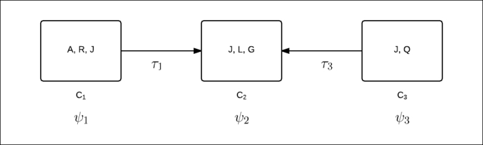
Fig 3.8: Message propagation from clusters and to cluster :

Now, let's consider another example, where we compute the probability of long queues (Q). We have to eliminate all the other random variables, except Q. Using the same approach as discussed earlier, first marginalize with respect to A and R, and compute as follows:

As discussed earlier, to eliminate the variable J, we need contributions from , , and , so we can't simply eliminate J from . The other two random variables L and G are only present in , so we can easily eliminate them from . However, to eliminate L and G from , we can't simply marginalize . We have to consider the contribution of (the outgoing message from ) as well, because J was present in both the clusters and . Thus, eliminating L and G would create as follows:

Finally, we can eliminate J by marginalizing the following belief of :

We can eliminate it as follows:

Fig 3.9 shows a message passing from to and to :

Fig 3.9: Message passing from to and to

In the previous examples, we saw how to perform variable elimination in a clique tree. This algorithm can be stated in a more generalized form. We saw that variable elimination in a clique tree induces a directed flow of messages between the clusters present in it, with all the messages directed towards a single cluster, where the final computation is to be done. This final cluster can be considered as the root. In our first example, the root was , while in the second example, it was . The notions of directionality and root also create the notions of upstream and downstream. If is on the path from to the root, then we can say that is upstream from , and is downstream from :

Fig 3.10: is upstream from and is downstream from

We also saw in the second example that was not able to send messages to until it received the message from , as the generation of also depends on . This introduces the notion of a ready cluster. A cluster is said to be ready to transmit messages to its upstream cliques if it has received all the incoming messages from its downstream cliques.

The message from the cluster j to the cluster i can be defined as the factor formed by the following sum product message passing computation:

We can now define the terms belief of a cluster . It is defined as the product of all the incoming messages from its neighbors with its own cluster potential:

Here, j is the upstream from i.

All these discussions for running the algorithm can be summarized in the following steps:

In the previous section, we discussed how to compute the probability of any variable using belief propagation. Now, let's look at the broader picture. What if we wanted to compute the probability of more than one random variable? For example, say we want to know the probability of long queues as well as a traffic jam. One naive solution would be to do a belief propagation in the clique tree by considering each cluster as a root. However, can we do better?

Consider the previous two examples we have discussed. The first one had as the root, while the other had . We saw that in both cases, message computed from the cluster to the cluster (that is ) is the same, irrespective of the root node. Generalizing this, we can conclude that the message from the cluster to the cluster will be the same as long as the root is on the side and vice versa. Thus, for a given edge in the clique tree between two clusters and , we have only two messages to compute, depending on the directionality of the edges ( and ). For a given clique tree with c clusters, we have edges between these clusters. Thus, we only need to compute messages.

As we have seen in the previous section, a cluster can propagate a message upstream as soon as it is ready, that is, when it has received all the incoming messages from downstream. So, we can compute both messages for each edge asynchronously. This can be done in two phases, one being an upward pass and the other being a downward pass. In the upward pass (Fig 3.11), we consider a cluster as a root and send all the messages to the root. Once the root has all the messages, we can compute its belief. For the downward pass (Fig 3.12), we can compute appropriate messages from the root to its children using its belief. This phase will continue until there is no message to be transmitted, that is, until we have reached the leaf nodes. This is shown in Fig 3.11:

Fig 3.11: Upward pass

Fig 3.11 shows an upward pass where cluster {E, F, G} is considered as the root node. All the messages from the other nodes are transmitted towards it.

The following figure shows a downward pass where the appropriate message from the root is transmitted to all the children. This will continue until all the leaves are reached:

Fig 3.12: Downward pass

When both, the upward pass and the downward pass are completed, all the adjacent clusters in the clique tree are said to be calibrated. Two adjacent clusters i and j are said to be calibrated when the following condition is satisfied:

In a broader sense, it can be said that the clique tree is calibrated. When a clique tree is calibrated, we have two types of beliefs, the first being cluster beliefs and the second being sepset beliefs. The sepset belief for a sepset can be defined as follows:

Until now, we have viewed message passing in the clique tree from the perspective of variable elimination. In this section, we will see the implementation of message passing from a different perspective, that is, from the perspective of clique beliefs and sepset beliefs. Before we go into details of the algorithm, let's discuss another important operation on the factor called factor division.

Factor division

A factor division between two factors and , where both X and Y are disjoint sets, is defined as follows:

Here, we define . This operation is similar to the factor product, except that we divide instead of multiplying. Further, unlike the factor product, we can't divide factors not having any common variables in their scope. For example, consider the following two factors:

a	b
		0
		1
		2
		3
		4
		5

b
	0
	1
	2

Dividing by , we get the following:

a	b
		0
		1
		1
		0
		4
		2.5

In pgmpy, factor division can implemented as follows:

In [1]: from pgmpy.factors import Factor
In [2]: phi1 = Factor(['a', 'b'], [2, 3], range(6))
In [3]: phi2 = Factor(['b'], [3], range(3))
In [4]: psi = phi1 / phi2
In [5]: print(psi)
╒═════╤═════╤════════════╕
│ a   │ b   │   phi(a,b) │
╞═════╪═════╪════════════╡
│ a_0 │ b_0 │     0.0000 │
├─────┼─────┼────────────┤
│ a_0 │ b_1 │     1.0000 │
├─────┼─────┼────────────┤
│ a_0 │ b_2 │     1.0000 │
├─────┼─────┼────────────┤
│ a_1 │ b_0 │     0.0000 │
├─────┼─────┼────────────┤
│ a_1 │ b_1 │     4.0000 │
├─────┼─────┼────────────┤
│ a_1 │ b_2 │     2.5000 │
╘═════╧═════╧════════════╛

Let's go back to our original discussion regarding message passing using division. As we saw earlier, for any edge between clusters and , we need to compute two messages and . Let's assume that the first message was passed from to , that is, . So, a return message from to would only be passed when has received all the messages from its neighbors.

Once has received all the messages from its neighbors, we can compute its belief as follows:

In the previous section, we also saw that the message from to can be computed as follows:

From the preceding mathematical formulation, we can deduce that the belief of , that is, , can't be used to compute the message from to as it would already include the message from to in it:

That is:

Thus, from the preceding equation, we can conclude that the message from to can be computed by simply dividing the final belief of , that is, , with the message from to , that is, :

Finally, the message passing algorithm using this process can be summarized as follows:

1. For each cluster , initialize the initial cluster belief as its cluster potential and sepset potential between adjacent clusters and , that is, as 1.
2. In each iteration, the cluster belief is updated by multiplying it with the message from its neighbors, and the sepset potential is used to store the previous message passed along the edge (), irrespective of the direction of the message.
3. Whenever a new message is passed along an edge, it is divided by the old message to ensure that we don't count this message twice (as we discussed earlier).

   Steps 2 and 3 can formally be stated in the following way for each iteration:

   
4. Here, we marginalize the belief to get the message passed. However, as we discussed earlier, this message will include a message from to in it, so divide it by the previous message stored in :
   
5. Update the belief by multiplying it with the message from its neighbors:
   
6. Update the sepset belief:
   
7. Repeat steps 2 and 3 until the tree is calibrated for each adjacent edge ():
   

As this algorithm updates the belief of a cluster using the beliefs of its neighbors, we call it the belief update message passing algorithm. It is also known as the Lauritzen-Spiegelhalter algorithm.

In pgmpy, this can be implemented as follows:

In [1]: from pgmpy.models import BayesianModel
In [2]: from pgmpy.factors import TabularCPD, Factor
In [3]: from pgmpy.inference import BeliefPropagation

# Create a bayesian model as we did in the previous chapters
In [4]: model = BayesianModel(
                      [('rain', 'traffic_jam'), 
                       ('accident', 'traffic_jam'),
                       ('traffic_jam', 'long_queues'), 
                       ('traffic_jam', 'late_for_school'),
                       ('getting_up_late', 'late_for_school')])

In [5]: cpd_rain = TabularCPD('rain', 2, [[0.4], [0.6]])
In [6]: cpd_accident = TabularCPD('accident', 2, [[0.2], [0.8]])
In [7]: cpd_traffic_jam = TabularCPD('traffic_jam', 2,
                                     [[0.9, 0.6, 0.7, 0.1],
                                      [0.1, 0.4, 0.3, 0.9]],                                                             
                                     evidence=['rain',
                                               'accident'],
                                     evidence_card=[2, 2])
In [8]: cpd_getting_up_late = TabularCPD('getting_up_late', 2,
                                         [[0.6], [0.4]])
In [9]: cpd_late_for_school = TabularCPD(
                         'late_for_school', 2,
                         [[0.9, 0.45, 0.8, 0.1], 
                          [0.1, 0.55, 0.2, 0.9]],
                         evidence=['getting_up_late','traffic_jam'],
                         evidence_card=[2, 2])
In [10]: cpd_long_queues = TabularCPD('long_queues', 2,
                                      [[0.9, 0.2], 
                                      [0.1, 0.8]],
                                      evidence=['traffic_jam'],
                                      evidence_card=[2])

In [11]: model.add_cpds(cpd_rain, cpd_accident, 
                        cpd_traffic_jam, cpd_getting_up_late,  
                        cpd_late_for_school, cpd_long_queues)

In [12]: belief_propagation = BeliefPropagation(model)

# To calibrate the clique tree, use calibrate() method
In [13]: belief_propagation.calibrate()

# To get cluster (or clique) beliefs use the corresponding getters
In [14]: belief_propagation.get_clique_beliefs()
Out[14]:
{('traffic_jam', 'late_for_school', 'getting_up_late'): <Factor representing phi(getting_up_late:2, late_for_school:2, traffic_jam:2) at 0x7f565ee0db38>,
 ('traffic_jam', 'long_queues'): <Factor representing phi(long_queues:2, traffic_jam:2) at 0x7f565ee0dc88>,
 ('traffic_jam', 'rain', 'accident'): <Factor representing phi(rain:2, accident:2, traffic_jam:2) at 0x7f565ee0d4a8>}

# To get the sepset beliefs use the corresponding getters 
In [15]: belief_propagation.get_sepset_beliefs()
Out[15]: {frozenset({('traffic_jam', 'long_queues'),
                    ('traffic_jam', 'rain', 'accident')}): <Factor 
representing phi(traffic_jam:2) at 0x7f565ee0def0>,
         frozenset({('traffic_jam', 'late_for_school', 
'getting_up_late'),
                   ('traffic_jam', 'long_queues')}): <Factor representing phi(traffic_jam:2) at 0x7f565ee0dc18>}

Querying variables that are not in the same cluster

In the previous section, we saw how to compute the probability of variables present in the same cluster. Now, let's consider a situation where we want to compute the probability of both being late for school (L) and long queues (Q). These two variables are not present in the same cluster. So, to compute their probabilities, one naive approach would be to force our clique tree to have these two variables in the same cluster. However, this clique tree is not the optimal one, hence it would negate all the advantages of the belief propagation algorithm. The other approach is to perform variable elimination over the calibrated clique tree.

The algorithm for performing queries of variables not present in same cluster can be summarized as follows:

1. Select a subtree of the calibrated clique tree , such that the query variable . Let be a set of factors on which variable elimination is to be performed. Select a cluster of the clique tree as the root node and add its belief to for each node in the clique tree except the root node.
   
2. Add it to . Let Z be a random set of random variables present in , except for the query variables. Perform variable elimination on the set of factors with respect to the variables Z.

In pgmpy, this can be implemented as follows:

In [15]: belief_propagation.query(
                         variables=['no_of_people'],                
                         evidence={'location': 1, 'quality': 1})
Out[15]: {'no_of_people': <Factor representing phi(no_of_people:2)
                                               at 0x7f565ee0def0>

MAP inference

Until now, we have been doing conditional probability queries only on the model. However, sometimes, rather than knowing the probability of some given states of variables, we might be interested in finding the states of the variables corresponding to the maximum probability in the joint distribution. This type of problem often arises when we want to predict the states of variables in our model, which is our general machine learning problem. So, let's take the example of our restaurant model. Let's assume that for some restaurant we know of, the quality is good, the cost is low, and the location is good, and we want to predict the number of people coming to the restaurant. In this case, rather than querying for the probabilities of states of the number of people, we would like to query for the state that has the highest probability, given that the quality is good, the cost is low, and the location is good. Similarly, in the case of speech recognition, given a signal, we are interested in finding the most likely utterance rather than the probability of individual phonemes.

Putting the MAP problem more formally, we are given a distribution defined by a set and an unnormalized , and we want to find an assignment whose probability is at maximum:

In the earlier equation, we used the unnormalized distribution to compute as it helps us avoid computing the full distribution, because computing the partition function Z requires all the values of the distribution. Overall, the MAP problem is to find the assignment for which is at maximum.

A number of algorithms have been proposed to find the most likely assignment. Most of these use local maximum assignments and graph structures to find the global maximum likely assignment.

We define the max-marginal of a function f relative to a set of variables Y as follows:

In simple words, returns the unnormalized probability value of the most likely assignment in . Most of the algorithms work on first computing this set of local max-marginals, that is , and then use this to compute the global maximum assignment, as we will see in the next sections.