
The Markov network doesn't give a very clear picture of the Gibbs parameterization of the distribution because we can't conclude whether the factors in it involve the maximal cliques or subgraphs. To overcome this limitation of the Markov network, we require a representation that can show the parameterization explicitly. The factor graph is one such representation.
A factor graph is a bipartite graph, one disjoint set being variable nodes, representing the variables, and the other being factor nodes, representing factors. An edge between a variable node and a factor node denotes that the random variable belongs to the scope of the factor. Thus, a factor graph is parameterized by a set of factors, where each of them is associated with a factor node, whose scope is all sets of all the random variables that it is neighbor to.
Generally, all the variable nodes are represented by a circle and all the factor nodes are represented by a square. Here's an example:
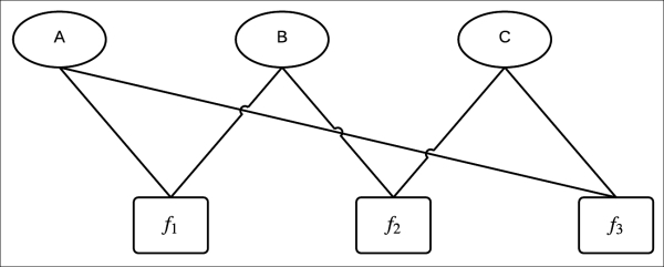
Fig 2.3 Factor graph
In the preceding factor graph, there are three variable nodes A, B, and C and three factor nodes associated with three factors, namely ![]() ,
, ![]() , and
, and ![]() . This representation is more explicit than the Markov network (Fig 2.4 (a)). From the Markov network, without checking the factors, we can't know whether the factors involve maximal clique (A, B, C) or their subgraphs {(A, B), (B, C), (C, A)}. This information is explicitly specified in the factor graph.
. This representation is more explicit than the Markov network (Fig 2.4 (a)). From the Markov network, without checking the factors, we can't know whether the factors involve maximal clique (A, B, C) or their subgraphs {(A, B), (B, C), (C, A)}. This information is explicitly specified in the factor graph.
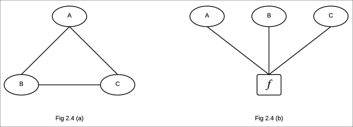
Fig 2.4 (a) Markov network of the corresponding factor graph in Fig 2.3
Fig 2.4 (b) Factor graph parameterized by factors involving maximal clique of the Markov network
In pgmpy, factor graphs can be created as follows:
# First import FactorGraph class from pgmpy.models
In [1]: from pgmpy.models import FactorGraph
In [2]: factor_graph = FactorGraph()

# Add nodes (both variable nodes and factor nodes) to the model
# as we did in previous other models
In [3]: factor_graph.add_nodes_from(['A', 'B', 'C', 'D',
                                     'phi1', 'phi2', 'phi3'])

# Add edges between all variable nodes and factor nodes
In [4]: factor_graph.add_edges_from(
                         [('A', 'phi1'), ('B', 'phi1'),
                          ('B', 'phi2'), ('C', 'phi2'),
                          ('C', 'phi3'), ('A', 'phi3')])
The FactorGraph class doesn't make any prior assumption about nodes; that is, it doesn't know which nodes are variable nodes and which nodes are factor nodes. It allows us to add edges between any nodes as long as they don't violate the bipartite nature of the factor graph. As soon as the bipartite property is violated by the addition of an edge, it raises the ValueError exception:
# We can also add factors into the model
In [5]: from pgmpy.factors import Factor
In [6]: import numpy as np
In [7]: phi1 = Factor(['A', 'B'], [2, 2], np.random.rand(4))
In [8]: phi2 = Factor(['B', 'C'], [2, 2], np.random.rand(4))
In [9]: phi3 = Factor(['C', 'A'], [2, 2], np.random.rand(4))
In [10]: factor_graph.add_factors(phi1, phi2, phi3)
We can also convert a Markov model into a factor graph and vice versa:
In [11]: from pgmpy.models import MarkovModel
In [12]: mm = MarkovModel()
In [13]: mm.add_nodes_from(['A', 'B', 'C'])
In [14]: mm.add_edges_from([('A', 'B'), ('B', 'C'), ('C', 'A')])
In [15]: mm.add_factors(phi1, phi2, phi3)
In [16]: factor_graph_from_mm = mm.to_factor_graph()

# While converting a markov model into factor graph, factor nodes
# would be automatically added the factor nodes would be in the
# form of phi_node1_node2_...

In [17]: factor_graph_from_mm.nodes()
Out[17]: ['C', 'B', 'phi_A_B', 'phi_B_C', 'phi_C_A', 'C']
In [18]: factor_graph.edges()
Out[18]: [('phi_A_B', 'A'), ('phi_A_C', 'A'), ('B', 'phi_B_C'),
          ('B', 'phi_A_B'), ('C', 'phi_B_C'), ('C', 'phi_C_A')]

# FactorGraph to MarkovModel

In [19]: phi = Factor(['A', 'B', 'C'], [2, 2, 2],

np.random.rand(8))
In [20]: factor_graph = FactorGraph()
In [21]: factor_graph.add_nodes_from(['A', 'B', 'C', 'phi'])
In [22]: factor_graph.add_edges_from(

                    [('A', 'phi'), ('B', 'phi'), ('C', 'phi')])
In [23]: mm_from_factor_graph = factor_graph.to_markov_model()
In [24]: mm_from_factor_graph.add_factors(phi)
In [24]: mm_from_factor_graph.edges()
Out[24]: [('B', 'A'), ('C', 'B'), ('C', 'A')]