
Let's try to do some inference tasks over the restaurant network in Fig 3.1. Let's say we want to find P(C). We know the following from the chain rule of probability:
Also, we know that the random variables L and Q are independent of each other if C is not observed. So, we can write the preceding equation as follows:
Now, we can see that we know the probability values involved in the product for the computation of P(C). We have the values of ![]() from the CPD of C, the values of P(l) from the CPD of L, and the values of P(q) from the CPD of Q. Summing up the product of these probabilities, we can easily find the probability of C.
from the CPD of C, the values of P(l) from the CPD of L, and the values of P(q) from the CPD of Q. Summing up the product of these probabilities, we can easily find the probability of C.
We can also note that the computational cost for this computation would be ![]() , where
, where ![]() represents the number of states of the variable X. We can see that in order to compute the probability of each state of C, we need to compute the product for each combination of states L and Q, and then add them together. This means that for each state of C, we have
represents the number of states of the variable X. We can see that in order to compute the probability of each state of C, we need to compute the product for each combination of states L and Q, and then add them together. This means that for each state of C, we have ![]() products and
products and ![]() additions. Here, 2 appears in the number of products because there are two product operations in the equation. Also, we need to do this computation
additions. Here, 2 appears in the number of products because there are two product operations in the equation. Also, we need to do this computation ![]() times for each state of C.
times for each state of C.
Now, let's take the example of another simple model ![]() and try to find P(D). We can find P(D) simply as follows:
and try to find P(D). We can find P(D) simply as follows:
However, we can see that the complexity of computing the values of P(D) is now ![]() , and for much more complex models, our complexity will be too high. Now, let's see how we can use the concept of dynamic programming to avoid computing the same values multiple times and to reduce our complexity. To see the scope of using dynamic programming in this problem, let's first simply unroll the summation and check what values we are computing. For simplicity, we will assume that each of the variables has only two states. Unrolling the summation, we get the following:
, and for much more complex models, our complexity will be too high. Now, let's see how we can use the concept of dynamic programming to avoid computing the same values multiple times and to reduce our complexity. To see the scope of using dynamic programming in this problem, let's first simply unroll the summation and check what values we are computing. For simplicity, we will assume that each of the variables has only two states. Unrolling the summation, we get the following:
![]() =
= ![]()
![]()
![]()
![]()
![]()
![]()
![]()
![]()
![]()
![]()
![]()
![]()
![]()
![]()
![]()
![]()
![]()
To calculate P(D), we must calculate ![]() and
and ![]() separately. After unrolling the summations, we can see that we have many computations that we have been doing multiple times if we take the simple linear approach. In the preceding equations, we can see that we have computed
separately. After unrolling the summations, we can see that we have many computations that we have been doing multiple times if we take the simple linear approach. In the preceding equations, we can see that we have computed ![]() four times,
four times, ![]() four times, and so on. Let's first group these computations together:
four times, and so on. Let's first group these computations together:
![]()
![]()
![]()
![]()
![]()
![]()
![]()
![]()
![]()
![]()
Now, replace these with symbols that we will compute only once and use them everywhere. Replacing ![]() with
with ![]() and
and ![]() with
with ![]() , we get:
, we get:
![]()
![]()
![]()
![]()
![]()
![]()
![]()
![]()
![]()
![]()
Again, grouping common parts together, we get:
![]()
![]()
![]()
![]()
![]()
![]()
Now, replacing ![]() with
with ![]() and replacing
and replacing ![]() with
with ![]() , we get:
, we get:
![]()
![]()
![]()
![]()
![]()
![]()
Notice how, instead of doing a summation over the complete product of ![]() here, we did the summation over parts of it:
here, we did the summation over parts of it:
Here, we have been able to push the summations inside the equation because not all the terms in the equation have all the variables. So, only the terms P(a) and P(b|a) depend on A. So we can simply sum them over the values of A.
To make things clearer, let's see another run of variable elimination on the restaurant model:
|
Step |
Variable eliminated |
Factors involved |
Intermediate factor |
New factor |
|---|---|---|---|---|
|
1 |
L |
|
|
|
|
2 |
Q |
|
|
|
|
3 |
C |
|
|
|
|
4 |
N |
|
|
|
This method helps us to significantly reduce the computation required to compute the probabilities. In this case, we just need to compute ![]() , which requires two multiplications and two additions, and
, which requires two multiplications and two additions, and ![]() , which requires four multiplications and two additions. We can then compute P(D). Hence, we just need a total of 12 computations to compute P(D). However, in the case of computing P(D) from the joint probability distribution, we require 16 * 3 = 48 multiplications and 14 additions. Hence, we see that using variable elimination brings about huge improvement in the complexity of making the inference.
, which requires four multiplications and two additions. We can then compute P(D). Hence, we just need a total of 12 computations to compute P(D). However, in the case of computing P(D) from the joint probability distribution, we require 16 * 3 = 48 multiplications and 14 additions. Hence, we see that using variable elimination brings about huge improvement in the complexity of making the inference.
Now, let's see how to make the inference using variable elimination with pgmpy:
In [1]: from pgmpy.models import BayesianModel
In [2]: from pgmpy.inference import VariableElimination
In [3]: from pgmpy.factors import TabularCPD

# Now first create the model.
In [3]: restaurant = BayesianModel(
                               [('location', 'cost'),
                                ('quality', 'cost'),
                                ('cost', 'no_of_people'),
                                ('location', 'no_of_people')])
In [4]: cpd_location = TabularCPD('location', 2, [[0.6, 0.4]])
In [5]: cpd_quality = TabularCPD('quality', 3, [[0.3, 0.5, 0.2]])
In [6]: cpd_cost = TabularCPD('cost', 2,
                              [[0.8, 0.6, 0.1, 0.6, 0.6, 0.05],
                               [0.2, 0.1, 0.9, 0.4, 0.4, 0.95]],
                               ['location', 'quality'], [2, 3])
In [7]: cpd_no_of_people = TabularCPD(
                            'no_of_people', 2,
                            [[0.6, 0.8, 0.1, 0.6],
                             [0.4, 0.2, 0.9, 0.4]],
                             ['cost', 'location'], [2, 2])
In [8]: restaurant.add_cpds(cpd_location, cpd_quality,
                            cpd_cost, cpd_no_of_people)

# Creating the inference object of the model
In [9]: restaurant_inference = VariableElimination(restaurant)

# Doing simple queries over one or multiple variables.
In [10]: restaurant_inference.query(variables=['location'])
Out[10]: {'location': <Factor representing phi(location:2) at
                                                0x7fea25e02898>}
In [11]: restaurant_inference.query(
                         variables=['location', 'no_of_people'])
Out[11]: {'location': <Factor representing phi(location:2) at
                                                0x7fea25e02b00>,
          'no_of_people': <Factor representing phi(no_of_people:2)
                                             at 0x7fea25e026a0>}

# We can also specify the order in which the variables are to be
# eliminated. If not specified pgmpy automatically computes the
# best possible elimination order.
In [12]: restaurant_inference.query(variables=['no_of_people'],
               elimination_order=['location', 'cost',  'quality'])
Out[12]: {'no_of_people': <Factor representing phi(no_of_people:2)
                                               at 0x7fea25e02160>
We saw the case of making an inference when no condition was given. Now, let's take a case where some evidence is given; let's say we know that the cost of the restaurant is high and we want to compute the probability of the number of people in the restaurant. Basically, we want to compute ![]() . For this, we could simply use the probability theory and first compute
. For this, we could simply use the probability theory and first compute ![]() and then normalize this over N again to get
and then normalize this over N again to get ![]() and then compute
and then compute ![]() as:
as:

Now, the question is, how do we compute ![]() ? We first reduce all the factors involving C to
? We first reduce all the factors involving C to ![]() and then do our normal variable elimination.
and then do our normal variable elimination.
In pgmpy, we can simply pass another argument to the query method for evidence. Let's see how to find ![]() using
using pgmpy:
# If we have some evidence for the network we can simply pass it
# as an argument to the query method in the form of
# {variable: state}
In [13]: restaurant_inference.query(variables=['no_of_people'],
                                    evidence={'location': 1})
Out[13]: {'no_of_people': <Factor representing phi(no_of_people:2)
                                               at 0x7fea25e02588>}
In [14]: restaurant_inference.query(
                      variables=['no_of_people'],
                      evidence={'location': 1, 'quality': 1})
Out[14]: {'no_of_people': <Factor representing phi(no_of_people:2)
                                               at 0x7fea25e02d30>}
# In this case also we can simply pass the elimination order for
# the variables.
In [15]:restaurant_inference.query(
                      variables=['no_of_people'],
                      evidence={'location': 1},
                      elimination_order=['quality', 'cost'])
Out[15]: {'no_of_people': <Factor representing phi(no_of_people:2)
at 0x7fea25e02eb8>}We have already seen that variable elimination is much more efficient for calculating probability distributions than normalizing and marginalizing the joint probability distribution. Now, let's do an exact analysis to find the complexity of variable elimination.
Let's start by putting the variable elimination algorithm in simple terms. In variable elimination, we start by choosing a variable ![]() , then we compute the factor product
, then we compute the factor product ![]() for all the factors involving that variable, and then eliminate that variable by summing it up, resulting in a new factor
for all the factors involving that variable, and then eliminate that variable by summing it up, resulting in a new factor ![]() whose scope is
whose scope is ![]() .
.
Now, let's consider that we have a network with n variables and m factors. In the case of a Bayesian network, the number of CPDs will always be equal to the number of variables, therefore, m = n for a Bayesian network. However, in the case of a Markov network, the number of factors can be more than the number of variables in the network. For simplicity, let's assume that we will be eliminating all the variables in the network.
In variable elimination, we have been performing just two types of operations, multiplication and addition. So, to find the overall complexity, let's start by counting these operations. For the multiplication step, we multiply each of the initial m factors and the intermediately formed n factors exactly once. So, the total number of multiplication steps would be ![]() , where
, where ![]() is the size of the intermediate factor
is the size of the intermediate factor ![]() . Also, let's define
. Also, let's define ![]() . Therefore,
. Therefore, ![]() will always be true. Now, if we calculate the total number of addition operations, we will be iterating over each of the
will always be true. Now, if we calculate the total number of addition operations, we will be iterating over each of the ![]() once, resulting in a total of
once, resulting in a total of ![]() addition operations. So, we see that the total number of operations for Variable Elimination comes out to be
addition operations. So, we see that the total number of operations for Variable Elimination comes out to be ![]() . Hence, the complexity of the overall operation is
. Hence, the complexity of the overall operation is ![]() , because
, because ![]() .
.
Now, let's try to analyze the variable elimination algorithm using the graph structure. We can treat a Bayesian model as a Markov model having undirected edges between all the variables in each of the CPD defining the parameters of the network. Now, let's try to see what happens when we run variable elimination over this network. We choose any variable X and multiply all other factors involving that factor X, resulting in a factor ![]() with the scope
with the scope ![]() . After this, we eliminate the variable X and have a resulting factor
. After this, we eliminate the variable X and have a resulting factor ![]() with scope
with scope ![]()
![]() . Now, as we have a factor with scope Y, we need to have edges in the network between each of the variables in Y. So, we add extra edges to the network, which are known as fill edges. For the elimination of the next variable, we use this new network structure and perform similar operations on it.
. Now, as we have a factor with scope Y, we need to have edges in the network between each of the variables in Y. So, we add extra edges to the network, which are known as fill edges. For the elimination of the next variable, we use this new network structure and perform similar operations on it.
Let's see an example on our late-for-school model showing the graph structure during the various steps of variable elimination:

Fig 3.2(a): Initial state of the network
Fig 3.2(b): After eliminating Traffic Accident (A)

Fig 3.2(c): After eliminating Heavy Rain (R)
Fig 3.2(d): After eliminating Traffic Jam (J)
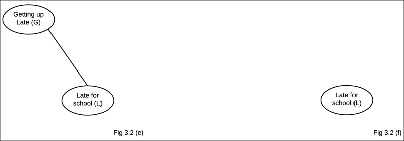
Fig 3.2(e): After eliminating Long Queues (Q)
Fig 3.2(f): After eliminating Getting Up Late (G)
An induced graph is also defined as the undirected graph constructed by the union of all the graphs formed in each step of variable elimination on the network. Fig 3.3 shows the induced graph for the preceding variable elimination:

Fig 3.3: The induced graph formed by running the preceding variable elimination
We can also check the induced graph using pgmpy:
In [16]: induced_graph = restaurant_inference.induced_graph(
                 ['cost', 'location', 'no_of_people', 'quality'])
In [17]: induced_graph.nodes()
Out[17]: ['location', 'quality', 'cost', 'no_of_people']
In [18]: induced_graph.edges()
Out[18]:
[('location', 'quality'),
 ('location', 'cost'),
 ('location', 'no_of_people'),
 ('quality', 'cost'),
 ('quality', 'no_of_people'),
('cost', 'no_of_people')]In variable elimination, the order in which we eliminate the variables has a huge impact on the computational cost of running the algorithm. Let's look at the difference in the elimination ordering on the late-for-school model. The steps of variable elimination with the elimination order A, G, J, L, Q, R are shown in the following table:
|
Step |
Variable eliminated |
Factors involved |
Intermediate factors |
New factor |
|---|---|---|---|---|
|
1 |
A |
|
|
|
|
2 |
G |
|
|
|
|
3 |
J |
|
|
|
|
4 |
L |
|
|
|
|
5 |
Q |
|
|
|
|
6 |
R |
|
|
|
The steps of variable elimination with the elimination order R, Q, L, J, G, A are shown in the following table:
|
Step |
Variable eliminated |
Factors involved |
Intermediate factors |
New factor |
|---|---|---|---|---|
|
1 |
R |
|
|
|
|
2 |
Q |
|
|
|
|
3 |
L |
|
|
|
|
4 |
J |
|
|
|
|
5 |
G |
|
|
|
|
6 |
A |
|
|
|
For every intermediate factor, we add filled edges between all the variables in their scope, so we can say that every intermediate factor introduces a clique in the induced graph. Hence, the scope of every intermediate factor generated during the variable elimination process is a clique in the induced graph. Also, notice that every maximal clique in the induced graph is the scope of some intermediate factor generated during the variable elimination process. Therefore, having a larger maximal clique in the induced graph also means having a larger intermediate factor, which means higher computation cost.
Let's see a few definitions related to induced graphs:
We have seen how the computation complexity of the variable elimination operation relates to the choice of elimination order, and how this relates to the tree width of the induced graph. A smaller tree width ensures a better complexity compared to an elimination order with a higher tree width. So, our problem has now been reduced to selecting an elimination order that keeps the tree width minimal.
Unfortunately, finding the elimination for the minimal tree width is NP -complete, so there is no easy way to find the complexity of the inference over a network by simply looking at the network structure. However, there are many other techniques that we can use to find good elimination orderings.
We define a graph as being chordal if it contains no cycle of length greater than three, and if there are no edges between two nonadjacent nodes of each cycle. In other words, every minimal cycle in a chordal graph is three in length.
Now, if you look carefully, you will see that every induced graph is a chordal graph. Also, the converse of this theorem holds, that every chordal graph on these variables corresponds to some elimination ordering. The proof of both of these theorems is beyond the scope of this book.
So, to find the elimination order, we use the maximum cardinality search algorithm. In this algorithm, we basically iterate ![]() times, and in each iteration, we try to find the variable with the largest number of marked variables and then mark that variable. This results in elimination ordering.
times, and in each iteration, we try to find the variable with the largest number of marked variables and then mark that variable. This results in elimination ordering.
Another approach to find elimination ordering is to take the greedy approach and, in each step, select a variable that seems to be the best option for that step. So, for each iteration, we compute a cost function to eliminate each of the nodes and select the node that results in the minimum cost. Some of the cost criteria are as follows:
- Min-neighbors: The cost of a node is defined by the number of neighbors it has in the graph.
- Min-weight: The cost of a node is the product of the cardinality of its neighbors.
- Min-fill: The cost of node elimination is the number of edges that need to be added to the graph for the elimination of that node.
- Weighted-min-fill: The cost of node elimination is the sum of the weights of the edges that need to be added to the graph for its elimination. The weight of an edge is defined as the product of the weights of the nodes between which it lies.
Here, we have seen two different approaches to finding good elimination ordering. The second heuristic approach of going the greedy way doesn't seem to be a very good approach to get globally optimized elimination ordering. However, it turns out that it gives very good results in most of the cases as compared to our maximum cardinality search algorithm.